Kansas Geological Survey, Open-file Report 93-48
KGS Open File Report 93-48
Prepared for presentation at The American Geophysical Union Fall Meeting
December 1993
The full report is available as an Adobe Acrobat PDF file (204 kB).
Spatial variations in the physical properties of an aquifer are a major control on the transport of contaminants in groundwater. In order to accurately predict the movement of pollutants in the subsurface, it is necessary to understand the factors controlling their transport. This research, which is an extension of earlier work by Taylor and Molz (1990), attempts to identify vertical variations in horizontal hydraulic properties at a relatively small scale using single-well tracer tests. With detailed data from several wells, an estimate of the lateral continuity of units with similar hydraulic properties can be made. Once the spatial distribution of hydraulic properties is better understood, contaminant movement in the subsurface can be predicted with more confidence. This presentation will outline the general method of tracer test data analysis and discuss its application, constraints, and results.
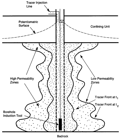
Four single-well tracer tests were conducted at a research site of the Kansas Geological Survey located near Lawrence, Kansas. The bedrock at the site, a consolidated silty sandstone, is overlain by approximately 22 m of unconsolidated Kansas River alluvium. The alluvium is composed of 11 m of sand and gravel overlain by 11 m of clay and silt overbank deposits. The sand and gravel interval, the focus of this study, is composed of sediment thought to be deposited by point-bar accretion. The underlying bedrock and the overlying silt and clay interval hydraulically restrict the sand and gravel aquifer, forming a leaky confined system. The four wells chosen for the tracer tests are fully screened in the sand and gravel interval.
This method, first reported in the groundwater literature by Taylor and Molz (1990), involves the injection of a nonreactive, electrically conductive tracer into a well under artificially induced, steady-state flow conditions (Figure 1). As the tracer solution enters the aquifer through the well screen, it moves radially outward from the well, displacing the native pore fluid. Since the electrical conductivity of a formation is predominantly controlled by porosity and pore fluid chemistry (Dobrin and Savit, 1988), a significant increase in the formation conductivity occurs as the tracer advances outward from the borehole. The invasion of the tracer is monitored by repeated induction logs using a recording interval of 3 cm. The rate of invasion as a function of depth can be determined from the induction logs. Detailed vertical profiles of effective porosity and hydraulic conductivity can then be constructed using the tracer invasion rates, the induced hydraulic gradient, and the observed change in formation electrical conductivity as the tracer invades the aquifer.
Figure 1--Tracer Injection
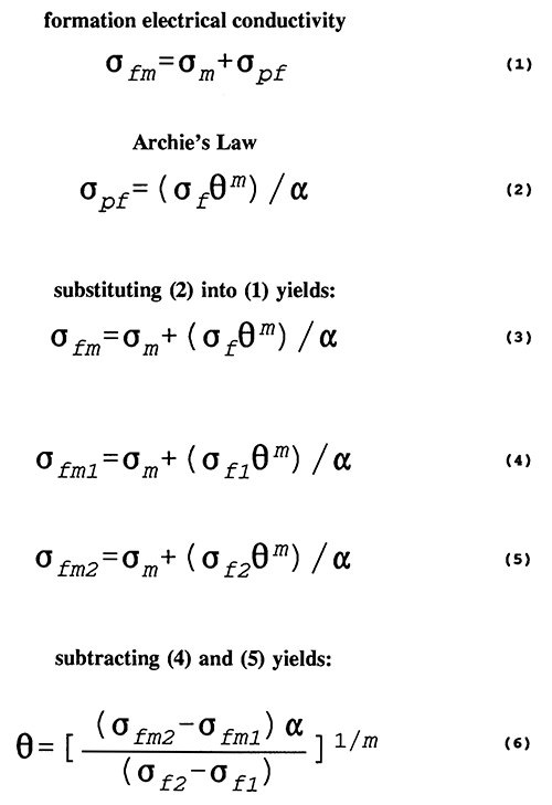
σfm = σm + σpf (1)
The contribution from the pore fluid can be represented by Archie's Law, Equation 2:
σpf = (σfφm) / α (2)
where φ = porosity, σpf = electrical conductivity of the pore fluid, α = tortuosity, and m = cementation factor.
Substituting Archie's Law into the model yields Equation 3:
σfm = σm + (σfφm) / α (3)
From the induction logs taken before tracer injection and those taken after the tracer has exceeded the radial detection of the tool, we know the formation conductivity when the aquifer is saturated with pore fluid of two different electrical conductivities. This allows Equation 3 to be written as 2 equations, Equations 4 and 5:
σfm1 = σm + (σf1φm) / α (4)
σfm2 = σm + (σf2φm) / α (5)
where σfm1 and σfm2 are the formation conductivity before and after tracer saturation, and σf1 and σf2 are the conductivity of the native pore water and the tracer solution, respectively. Subtracting Equation (4) from (5) and solving for porosity yields Equation 6:
φ = [ (σfm2 - σfm1)α / (σf2 - σf1) ] 1/m (6)
The cementation factor, m, and tortuosity, α, are dependant on lithology and pore structure. It has been shown that for unconsolidated sands, these variables are approximately 1.4 and 1.0, respectively (Jackson et al., 1978).
Figure 2--Estimation of Effective Porosity
The radius of tracer invasion is determined for each induction log using the radial dependence of the induction tool. The formation conductivity at a single interval is a weighted vertical and horizontal average of the conductivity of the formation adjacent to that interval. The relation between magnitude of contribution and radial distance from the borehole is called the radial response function. Figure 3 is a plot of the cumulative sum of the radial responses. This plot is a function of the coil geometry of the particular induction tool used.
Figure 3--Radial Dependence of the Induction Tool
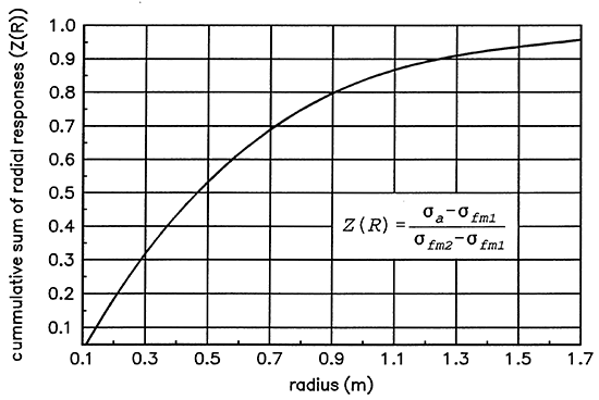
The cumulative sum of the radial responses, Z(R), is a ratio defined on Figure 3:
Z(R) = (σa - σfm1) / (σfm2 - σfm1) (7)
where σa is a formation electrical conductivity measured during tracer injection. Given σa, σfm1 and σfm2 the tracer front position is determined from Figure 3.
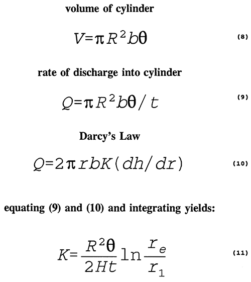
Knowing the radial position of the tracer front as a function of time, the hydraulic conductivity can be estimated by equating a simple geometric representation of radial plug flow and Darcy's Law (Taylor and Molz, 1990) (Figure 4).
The volume of pore fluid within a segment of an aquifer can be represented by a cylinder with the well at the center, as shown in Equation 8:
V = πR2bφ (8)
where V = volume, R = radius of cylinder, b = height of cylinder, and φ = porosity. The discharge into this volume is represented by Equation 9:
Q = πR2bφ / t (9)
where Q = discharge, and t = time since initiation of tracer injection.
Discharge into this segment can also be represented by Darcy's law, Equation 10:
Q = 2πrbK(dh/dr) (10)
Equating Equations 9 and 10, integrating, and solving for K yields Equation 11:
K = (R2φ / 2Ht) ln (re / r1) (11)
where H = induced hydraulic head in injection well, re = effective radius (radius beyond which aquifer head is at static), and r1 = radius of the injection well. Given the porosity and the position of the tracer front, Equation 11 is used to estimate a value of hydraulic conductivity at each interval from an induction log.
Figure 4--Estimation of Hydraulic Conductivity
This method of parameter estimation appears to be theoretically sound. However, due to aquifer non-idealities, modification of this approach is required to accurately estimate aquifer hydraulic parameters. In some cases, these non-idealities lead to the violation of assumptions fundamental to the application of the model. If this occurs, the method may fail to accurately estimate the parameters.
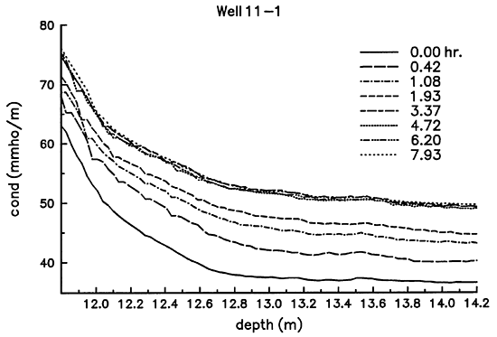
The method of Taylor and Molz assumes tracer injection continues until the tracer displaces all of the native pore water within the radius of detection of the induction tool. When the tracer exceeds this radius, repeat induction logs show no change with time. Figure 5 contains several logs of formation conductivity during tracer injection for an interval in well 11-1. As the tracer solution displaces the native pore water, the formation conductivity increases. After time 3.37 hr., the formation conductivity does not change, suggesting complete invasion has occurred. In this interval, effective porosity can be estimated from the formation conductivity measured before and after tracer invasion.
Figure 5--Formation Conductivity During Tracer Injection
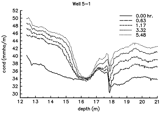
In low permeability intervals, the rate of tracer invasion may be very slow. As a result, the tracer solution may not reach the radius of detection of the induction tool within a reasonable time. Figure 6 contains several logs of formation conductivity taken during tracer injection in well 5-l. The formation conductivity in the interval from 16 to l7 m shows only a small change during tracer injection, suggesting minimal tracer invasion. since complete invasion has not occurred, an accurate value of formation conductivity with tracer saturation cannot be measured, and an estimate of effective porosity cannot be made.
Figure 6--Formation Electrical Conductivity During Tracer Injection
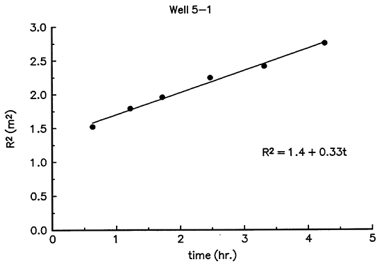
This method of analysis also has problems if a disturbed zone (or skin) exists adjacent to the well. The radial response function used to determine the tracer front position is a cumulative sum of the contributions of formation conductivity from all zones within the radius of detection of the induction tool. Thus, the contribution of formation conductivity from the disturbed zone will influence every estimate of the extent of tracer invasion. As a result, all estimates of tracer invasion will be shifted by a constant factor that is a function of the hydraulic properties and size of the disturbed zone. Note that Equation 11 (Figure 4) defines a linear relationship between the radius of tracer invasion-squared and time; a straight line fit to a plot of radius-squared versus time should pass through the origin, as shown in Figure 7. However, in the presence of a skin, this line is shifted by a constant factor, producing a nonzero y-intercept. Figure 8 is a plot of radius-squared versus time from an interval in well 5-1. The positive shift displays an overestimation of radius-squared, identifying the existence of a high-permeability or -porosity skin. This shift in radius squared will produce a time dependance in the hydraulic conductivity values estimated from Equation 11. However, if the individual values for radius-squared and time in this equation are replaced with the slope of radius-squared versus time, the influence of the shift produced by the skin will be eliminated.
Figure 7--R2 Versus t at Depth of 20.48 m.
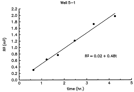
Figure 8--R2 Versus t at Depth of 14.02 m.
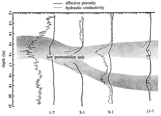
Employing the Taylor and Molz method for porosity estimation where appropriate and the slope method for hydraulic conductivity estimation, interesting results were obtained from the four tracer tests. Natural gamma and induction logs from this site prior to the tracer tests do not identify any correlatable structures in the sand and gravel interval. However, porosity and hydraulic conductivity profiles determined from these tests identify significant correlatable zones with variations in porosity of a factor of 2 and variations in hydraulic conductivity of 2 orders of magnitude. Figure 9 is a profile of relative effective porosity and hydraulic conductivity from the sand and gravel interval determined from the four tracer tests. (The lateral distance spanned by the string of wells is 30.5 m.) The most notable feature is the central low permeability zone. Wells 11-1 and 9-1 display two low permeability zones separated by a higher permeability zone. This higher permeability zone pinches out and is not present in wells 5-1 and 1-7. Spatial variations in hydraulic properties of this magnitude may significantly influence the migration of contaminants. These variations must be quantified if attempts to model this system are to be successful.
Figure 9--Profiles of Relative Effective Porosity and Hydraulic Conductivity
The capability of this tracer test method to quantify spatial variations on a relative scale is quite good. However, the absolute magnitude of the hydraulic conductivity estimates is too low. The estimated values for hydraulic conductivity are over an order of magnitude lower than those obtained by core analyses and slug and pumping tests at this site. The reason for this discrepancy is unclear at this time, but it may be partly related to an error in the definition of the radial response function for our induction tool. Further research is necessary before a complete evaluation of the field method can be made.
In conclusion, the borehole induction tracer test appears to have great potential for the identification of spatial variations in hydraulic parameters. Refinements have been made such that the method can be used for wells with both high and low permeability skins. A major component of future research on this approach will focus on the method's ability to provide better estimates of the actual magnitude of the hydraulic parameters.
Dobrin, M.B., and Savit, C.H., 1988, Introduction to Geophysical Prospecting. McGraw-Hill, Inc., New York, NY, 842 p.
Jackson, P.O., Taylor-Smith, D. and Stanford, P.N., 1978, Resistivity-porosity-particle shape for marine sands: Geophysics, v. 43, no. 6, pp. 1250-1268.
Taylor, K. and Molz, F., 1990, Determination of hydraulic conductivity and porosity logs in wells with a disturbed annulus: Journal of contaminant Hydrology, no. 5, pp. 317-332.
This research was financed in part by the Air Force Office of scientific Research, Air Force Systems Command, U.S.A.F., under grant number AFOSR 91-0298 to C. D. McElwee and J. J. Butler, Jr. The contents of this document do not necessarily represent the views or policies of the U.S.A.F., nor does mention of commercial products constitute their endorsement by the U.S.A.F.
Assistance for the illustration of figures in this document was provided by Mark Schoneweis of the Kansas Geological Survey.
Kansas Geological Survey, Geohydrology
Placed online May 12, 2015; originally released Dec. 1993
Comments to webadmin@kgs.ku.edu
The URL for this page is http://www.kgs.ku.edu/Hydro/Publications/1993/OFR93_48/index.html