Kansas Geological Survey, Open-file Report 91-63
KGS Open File Report 91-63
Prepared for the Fall 1991 AGU Meeting San Francisco, CA
Also available as an Acrobat PDF file.
Slug tests are commonly used for site characterization. An earlier paper (EOS, v. 70, no. 43, p. 1078) dealt with the use of sensitivity analysis to design a test which would give reasonably accurate estimates of the aquifer parameters by an informed choice of the number and times of measurements. Most practitioners know that slug tests are not very sensitive to the storage coefficient, as explained in the earlier paper. An investigation of the radial dependence of the Cooper et al. (1967) analytical slug test solution shows that the use of one or more observation wells can vastly improve the parameter estimates, particularly the estimate for storage. While it would usually not be practical to install an observation well solely for use in a slug test, many times nearby wells are available. Generally, the observation well must be fairly close (a few tens of feet or less) to the slugged well to be effective. The storage coefficient must be small in order to see the effect of the slug at greater distances from the slugged well. Since the temporal and spatial dependence of the sensitivities for transmissivity and storage are considerably different, the addition of one or more observation wells will substantially reduce the correlation between these two parameters, and result in much better estimates than usually obtained in slug tests. These ideas are illustrated using typical data from our research sites.
Slug tests are commonly used for site characterization. An earlier paper (EOS, v. 70, no. 43, p. 1078) dealt with the use of sensitivity analysis to design a test which would give reasonably accurate estimates of the aquifer parameters by an informed choice of the number and times of measurements. Most practitioners know that slug tests are not very sensitive to the storage coefficient, as explained in the earlier paper. An investigation of the radial dependence of the Cooper et al. (1967) analytical slug test solution shows that the use of one or more observation wells can vastly improve the parameter estimates, particularly the estimate for storage.
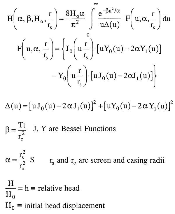
Slug-test responses can be expressed as a function of four parameters: alpha, a parameter related to screen and casing radii and the storage coefficient; beta, a dimensionless time involving transmissivity and the casing radius; Hn, the initial head displacement; and r/rS, the distance to an observation well divided by the screen radius.
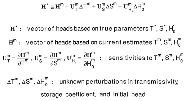
First Order Taylor Expansion for the Head
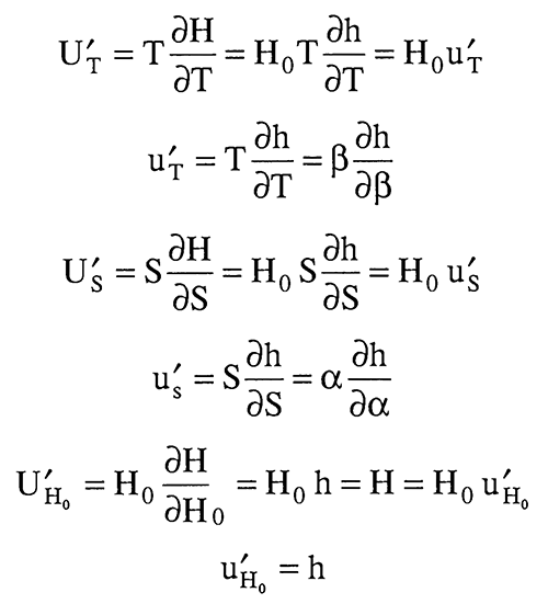
u't, u'S, and u'H0 are functions of α, β, and r/rS. We shall look at these functions in greater detail later.
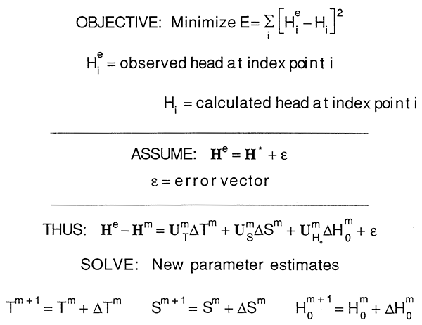
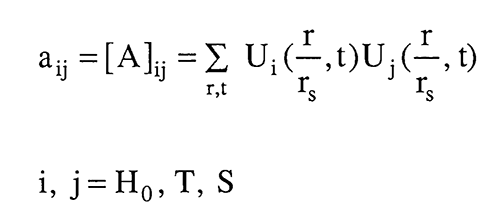
The sensitivity design matrix [A] defined here is a sum over time and space of products for any two sensitivity coefficients. If we are fitting all three parameters H0, T, and S then the sensitivity design matrix is 3 x 3. The least squares solution for the delta parameter changes can be expressed in terms of the inverse of [A]. In general, the solution is well behaved if the diagonal elements are large and nearly equal and the off-diagonal elements are small. This will be the case if the sensitivity coefficients are large and do not have similar shapes over the measurement times and locations.
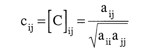
One way to measure the similarity of the sensitivity coefficients is to define the sensitivity correlation matrix as shown here; it will have ones on the diagonal and the off-diagonal terms will vary between ±1. If any of the off-diagonal terms are exactly one, the inverse of [A] does not exist and the inverse problem can not be solved for aquifer parameters. From a practical standpoint, anytime the off-diagonal elements of the correlation matrix get above .9 the [A] matrix becomes ill-conditioned rather rapidly and the inverse solution becomes more unreliable.
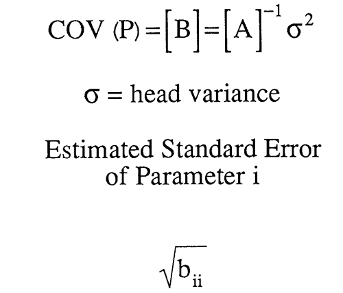
As long as an inverse of [A] can be found, the reliability of the parameter estimates can be assessed by looking at the parameter covariance matrix defined here. The form shown here results from some simplifying assumptions about the errors in head such as additive, zero mean, noncorrelated and constant variance. With these assumptions the estimated standard errors of the parameters are given by the square roots of the diagonal elements of the parameter covariance matrix.
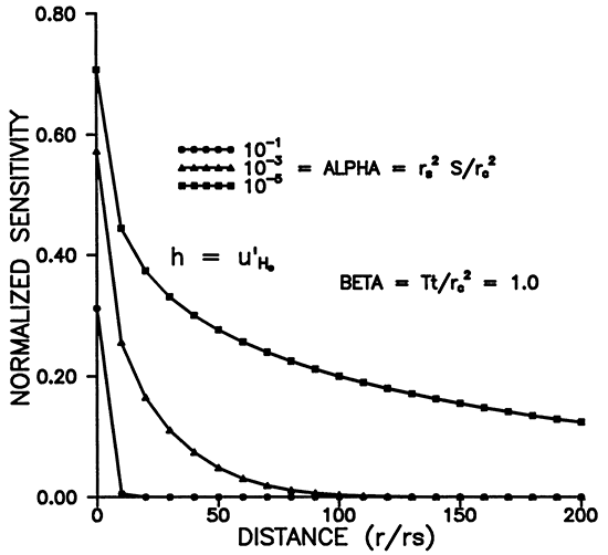
Figure 1 shows the relative head or sensitivity to H0, versus dimensionless time for various radii. The maximum occurs for r = rS (Figures 1 and 3), and decreases with time and distance. Figure 3 shows that the area of influence spreads with time. Figure 1 shows that an observation well will respond in time with a bell shaped curve whose maximum amplitude decays with distance from the slugged well. At about 175rS the response has fallen to about .01 H0 at a dimensionless time of 10 for α = 10-3 (Figures 1 and 2). Smaller α's result in larger responses in space and time as shown in Figures 2 and 4.
Figure 1--Variation of u'H0 with time for various r/rS.
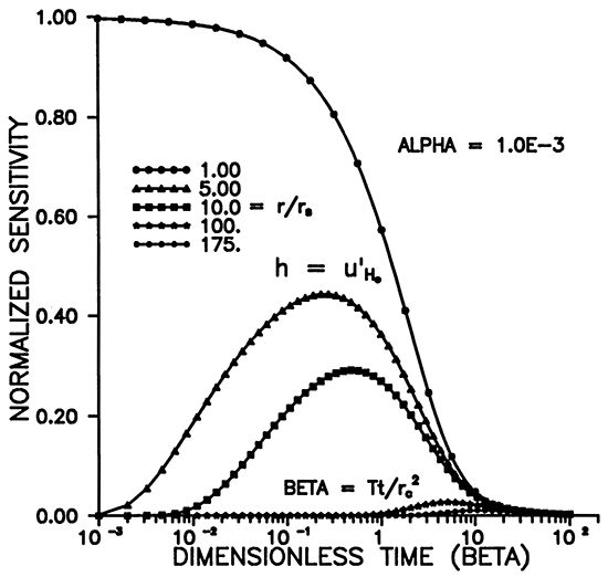
Figure 2--Variation of u'H0 with time for various alpha.
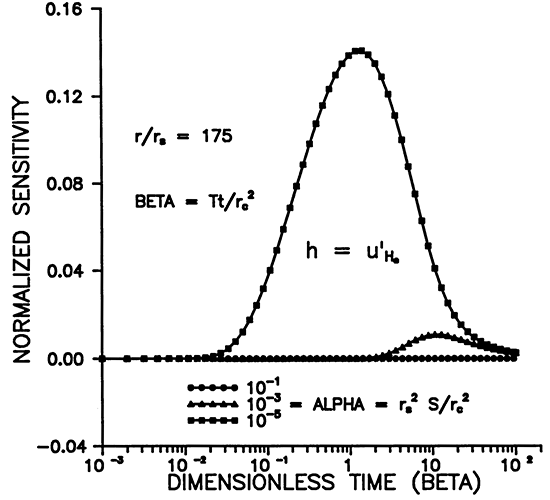
Figure 3--Variation of u'H0 with distance for various times.
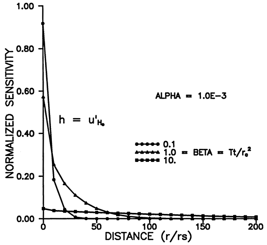
Figure 4--Variation of u'H0 with distance for various alpha.
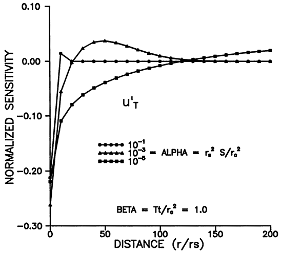
Figures 5-8 illustrate the dependence of the sensitivity to transmissivity on time, distance, and alpha. u'T has positive and negative lobes except for r = rS (Figures 5 and 7). Figure 7 shows that the maximum sensitivity to transmissivity occurs at the well. A given observation well will be sensitive to the transmissivity over a definite time interval (Figure 5), and the sensitivity decays rapidly with increasing r. Figures 6 and 8 illustrate the dependence on the storage coefficient (alpha). The maximum amplitude of the sensitivity seems to vary inversely with alpha (Figure 6), while the amplitude at r = rS does not seem to have a strong dependence on alpha (Figure 8). As noted previously, we need a smaller alpha (storage coefficient) for sensitivities to propagate farther from the slugged wells. (Figure 8).
Figure 5--Variation of u'T with time for various r/rS.
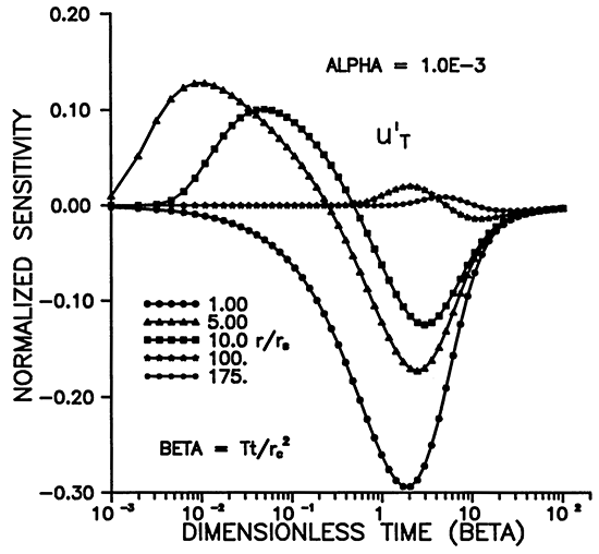
Figure 6--Variation of u'T with time for various alpha.
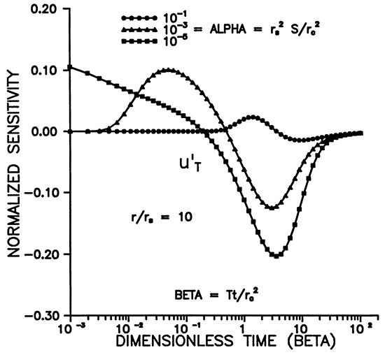
Figure 7--Variation of u'T with distance for various times.
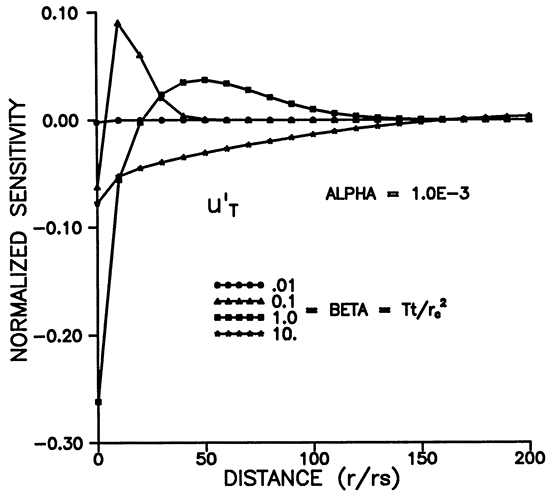
Figure 8--Variation of u'T with distance for various times.
Figures 9-12 illustrate the dependence of the sensitivity to storage on α, β, and r. The maximum sensitivity does not occur at r = rS (Figures 9 and 11), but rather at a distance of about 5rS for α = 10-3. Figure 11 shows that the shape of u'S moves out to larger distances while widening and decaying with increasing time. The dependence on alpha shown in Figure 12 reveals that the signal propagates much farther from the well for smaller values of α. Figure 10 shows that, for a chosen r, the maximum amplitude of the sensitivity is inversely proportional to α and occurs at earlier times for smaller α's.
Figure 9--Variation of u'S with with time for various r/rS.
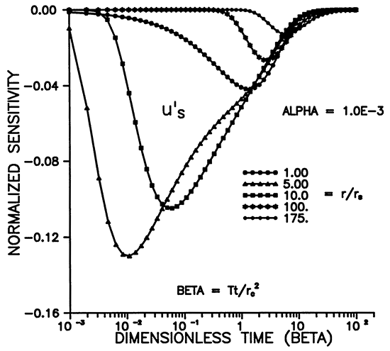
Figure 10--Variation of u'S with time for various alpha.
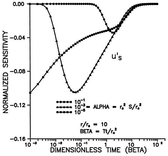
Figure 11--Variation of u'S with distance for various times.
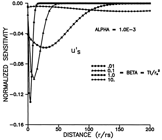
Figure 12--Variation of u'S with distance for various times.
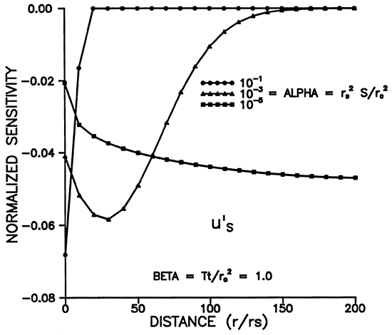
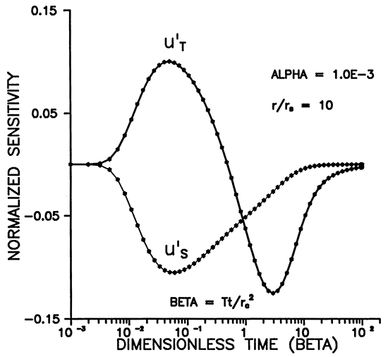
Figure 13 shows that the shape of the sensitivities with respect to transmissivity and storage at r = rS are extremely similar except for amplitude. This means that data from a slugged well are much more sensitive to T than S and that there will be high correlation between these two parameters. On the other hand, Figure 14 shows the two sensitivities at r = 10rS and reveals that they have considerably different shapes and nearly the same maximum amplitude. This means that the observation well is much more sensitive to storage and that the correlation between T and S is dramatically reduced by the use of an observation well.
Figure 13--Comparison of sensitivities at the screen radius.
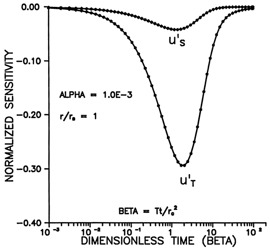
Figure 14--Comparison of sensitivities at 10 screen radii.
We have developed an alluvial field site for hydraulic testing. It consists of about 35 feet of coarse sand and gravel overlain by about 35 feet of silt and clay. The following is a simulation of expected results at this site. From earlier laboratory work and pumping tests we know some average values for K, T and S.
K ≈ 300 ft/day = .208 ft/min
T ≈ (.208 ft/min) (35 feet) = 7.28 ft2/min
S ≈ .00063
We simulate the results for the slugged well and two observation wells at 5 and 10 feet away, taking data over a three minute interval (slug tests are very short duration in this media). It is assumed the slugged well is 4 inches in diameter and all wells are fully screened. The N simulated data is rounded to the nearest tenth of a foot and then analyzed in an inverse program.
| Results | |||
|---|---|---|---|
| Slugged Well Only | Slugged Well + Obs. Well | Slugged Well + 2 Obs. Wells | |
| Range of T (ft2/min) |
7.11 - 8.00 | 7.22 - 7.37 | 7.24 - 7.38 |
| Range of S | (.178 - .722) x 10-3 | (.616 - .666) x 10-3 | (.609 - .648) x 10-3 |
| Corr. | .98 | .54 | .44 |
| rms Dev. | .026 | .026 | .025 |
| Remarks | Trouble Converging | Converged rapidly | Converged Rapidly |
As part of a regional study of the Dakota aquifer in Kansas a number of pumping and slug tests have been performed. One site in Lincoln County was slug tested with an observation well. The following are details of the two wells:
| Slugged Well | Observ. Well | |
|---|---|---|
| Depth | 98.4 feet | 94.4 feet |
| Dia. | 4 inches | 2 inches |
| Screen | 78-98 feet | 84-94 feet |
The test was analyzed three ways:
| Slugged Well | Obser. Well | Slugged Well + Obser. Well | |
|---|---|---|---|
| T (ft2/sec) | .896 X 10-3 | 1.0005 X 10⁻² | 1.029 X 10⁻² |
| S | .2 X 10-3 | .514 X 10-4 | .520 X 10-4 |
| Corr. | .99 | .269 | .49 |
| rms Dev | .0024 | .0030 | .0040 |
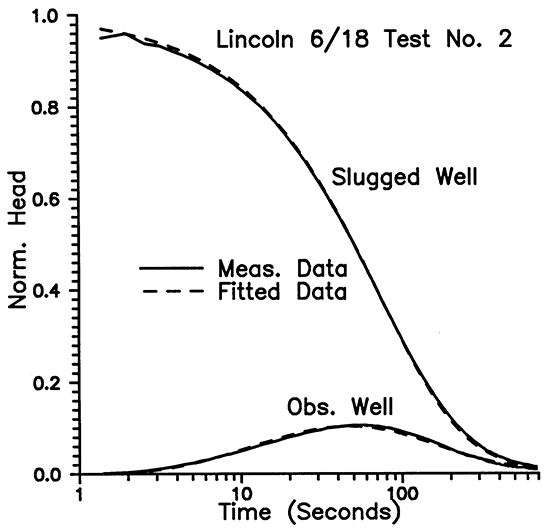
It is clear that the use of an observation well greatly improves the estimate for S and makes the inverse problem much better conditioned. Figure 15 shows the field measurements and the fitted data.
Figure 15--Dakota aquifer test, Lincoln County, Kansas.
While it would usually not be practical to install an observation well solely for use in a slug test, many times nearby wells are available. Generally, the observation well must be fairly close (a few tens of feet or less) to the slugged well to be effective. The storage coefficient must be small in order to see the effect of the slug at greater distances from the slugged well. Since the temporal and spatial dependence of the sensitivities for transmissivity and storage are considerably different, the addition of one or more observation wells will substantially reduce the correlation between these two parameters, and result in much better estimates than usually obtained in slug tests. These ideas have been illustrated using typical data from our research sites.
This research was sponsored in part by the Air Force Office of Scientific Research, Air Force Systems Command, USAF, under grant or cooperative agreement number, AFOSR 91-0298. This research was also supported in part by the U.S. Geological Survey (USGS), Department of the Interior, under USGS award number 14-08-0001-G2093. The views and conclusions contained in this document are those of the authors and should not be interpreted as necessarily representing the official policies, either expressed or implied, of the U.S. Government. The US Government is authorized to reproduce and distribute reprints for Governmental purposes notwithstanding any copyright notation thereon.
Kansas Geological Survey, Geohydrology
Placed online Jan. 23, 2015; originally released Dec. 1991
Comments to webadmin@kgs.ku.edu
The URL for this page is http://www.kgs.ku.edu/Hydro/Publications/1991/OFR91_63/index.html