Kansas Geological Survey, Open-file Report 91-62
KGS Open File Report 91-62
Prepared for the Fall 1991 AGU Meeting San Francisco, CA
Also available as an Acrobat PDF file.
Slug tests have become one of the more commonly employed techniques in applied hydrogeology. In this approach, estimates for subsurface flow properties are obtained through a comparison of the slug-test response data to various analytical solutions. The assumptions underlying the analytical solutions, however, limit their applicability to many typical field situations. We have developed a numerical model that allows the simulation of slug tests under conditions for which analytical solutions are not feasible. The model uses a finite difference approximation of the 3-D cylindrical flow equation, allowing an arbitrary spatial distribution of flow properties. An approximate representation of the wellbore itself is included in the model domain enabling flow in the immediate vicinity of the well to be studied in detail. In this presentation, the model will be used to assess the effects of horizontal layers of differing hydraulic conductivity on slug tests in confined aquifers. The nature of the vertical averaging of flow properties that occurs-in a slug test will be examined and the viability of multilevel slug tests will be discussed for a range of conditions.
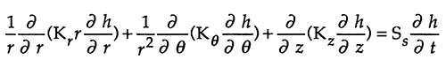
A finite difference numerical model is employed in this study to solve the 3-D, confined groundwater flow equation in cylindrical coordinates:
This model has been developed at the Kansas Geological Survey (Liu and Butler, 1992) to aid in research and analysis of many types of well tests (i.e. pumping tests, slug tests, etc). A very general approach has been used in model development in order to enable the model to be used to simulate a large variety of conditions. The model can also be configured in a continuous-time mode (Liu and Butler, 1991) so that drawdown data from a well test can be readily compared to simulated results. A simplistic representation of the well bore, based on earlier work of Rushton and Chan (1977) and Butler (1986), is also included in the model (see Section III). This feature allows slug tests and early times of pumping tests to be readily simulated.
To assess the viability of multilevel slug tests for identifying vertical variations in horizontal hydraulic conductivities, the numerical model was used to generate synthetic slug-test results under a number of test configurations. The tests were carried out using four different hypothetical aquifers: 1) uniform, isotropic; 2) uniform, anisotropic; 3) layered, isotropic; and 4) layered, anisotropic. The layered aquifers consist of alternating high and low conductivity layers, with the following radial (r) and vertical (z) conductivity values:
| anisotropic | isotropic | |
|---|---|---|
| low | Kr = 1; Kz = 0.1 | Kr = Kz = 1 |
| high | Kr = 10; Kz = 1 | Kr = Kz = 10 |
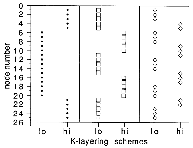
The uniform aquifers each consist of a single conductivity zone with the low-K properties given above. In all cases, the aquifer is 25 units thick (with each unit being represented by a single node in the vertical). The aquifer is bounded above and below by impermeable boundaries. In addition, a constant head boundary is present at an outer radius of 37364.15. The two layered aquifers (isotropic and anisotropic) are divided into five layers of five nodes each, alternating Klo, Khi, Klo, Khi, Klo, from top to bottom. (This is the layering scheme shown in the middle of figure 3.)
Other parameters employed are:
The simulations of multilevel slug tests all employ a well fully screened in the aquifer with a limited slugged interval isolated by packers above and below (double packer). A separate packer above the screen limits movement of water into the open sections of the well above the double packer. This configuration is similar to that described by Melville et al. (1991). The nodes representing the slugged interval are assigned an initial head of 1.0, while the remaining nodes in the model (including those in the screened section of the well outside the double packer) are assigned an initial head of 0. The entire wellbore is assigned extremely high hydraulic conductivities (Kr = Kz = 1 X 10⁷). Thus, the wellbore is simulated as a highly conductive zone.
The slugged interval is assigned a specific storage equal to the inverse of its length, so that the storage coefficient for the slugged interval equals 1.0. This implies that the volume of water released from the well for a given drop in head, Δh, is simply Δhπrw2. The open sections of wellbore outside the double packer are assigned a value for specific storage that corresponds to the compressibility of water, that is Ss = ρ g β where β is the compressibility of water. In metric units, the value of Ss for water is 4.312 X 10⁻⁶ m-1. Rigorously, specifying this value as the specific storage in the open sections of the wellbore fixes the distance units as meters. However, several test runs have shown that the results are quite insensitive to this value, so that the following results can be considered essentially dimensionless.
A number of runs revealed that the simulated slug test results are fairly insensitive to the length of the individual packers in the double packer, as long as they prevent vertical flow in the wellbore. The following results are obtained using packers which are two nodes long both above and below the slugged interval.
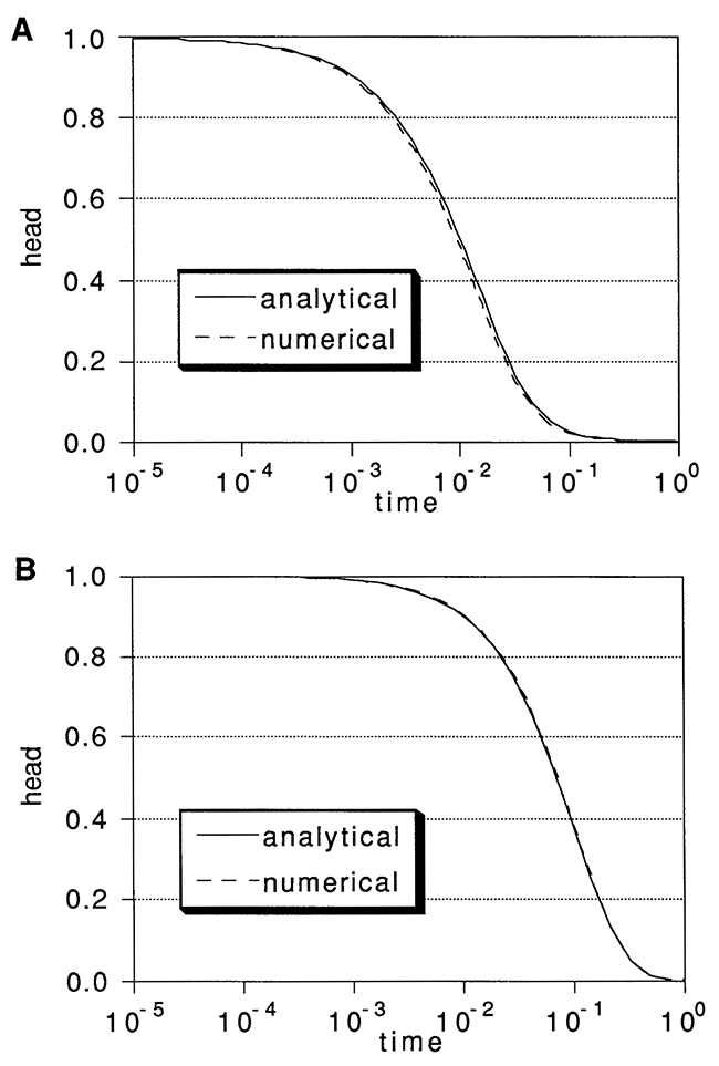
In order to assess the viability of this model for the examination of slug tests, a series of runs were made to compare model output with results from analytical solutions. Two examples from this series are given here. Figure 1A compares the model simulated results using a well with a fully open screen (25 units long) in the uniform, isotropic aquifer with those from the analytical solution of Cooper, Bredehoeft, and Papadopulos (CBP) (1967) for slug tests in fully penetrating aquifers. Figure 1B compares the model simulated results using a one-node long slugged interval in the uniform, isotropic aquifer with those from the analytical solution for multilevel slug tests developed by McElwee et al. (1990). In both cases, the model fits are quite good, with the majority of the model error being traceable to discretization in the radial direction. The discretization scheme employed here is good enough, however, for the purposes of this study.
Figure 1--Verification of numerical model for (A) fully penetrating case and (B) partially penetrating case.
One issue of considerable interest to researchers has been the type of average of aquifer flow properties that will result from using various hydraulic tests. Figure 2 displays the results for several simulations of slug tests in aquifers with the same thickness-weighted average of layer conductivities, but with different patterns of conductivity variations. Results are shown for the analytical CBP solution with Kr = 4.6, a one-K-zone numerical simulation with Kr = 4.6, Kz = 0.46, and three other simulations of layered aquifers with alternating bands of the properties Klo and Khi (table, page 2) for the layered, anisotropic aquifer. The layering schemes are shown in Figure 3. The middle scheme is the one used for the simulations of multilevel slug tests. All three layering schemes have a thickness weighted average Kr of 4.6 (15 units of Kr = 1.0 and 10 units of Kr = 10.0) and a thickness weighted average Kz of 0.46 (15 units of Kz = 0.1 and 10 units of Kz = 1.0).
Figure 2--Effects of variable layering on fully-penetrating slug test results at (A) the slugged well and (B) an observation well located at vertical node 13 and 3.7 units radial distance from the slugged well. Layering schemes are shown in Figure 3.
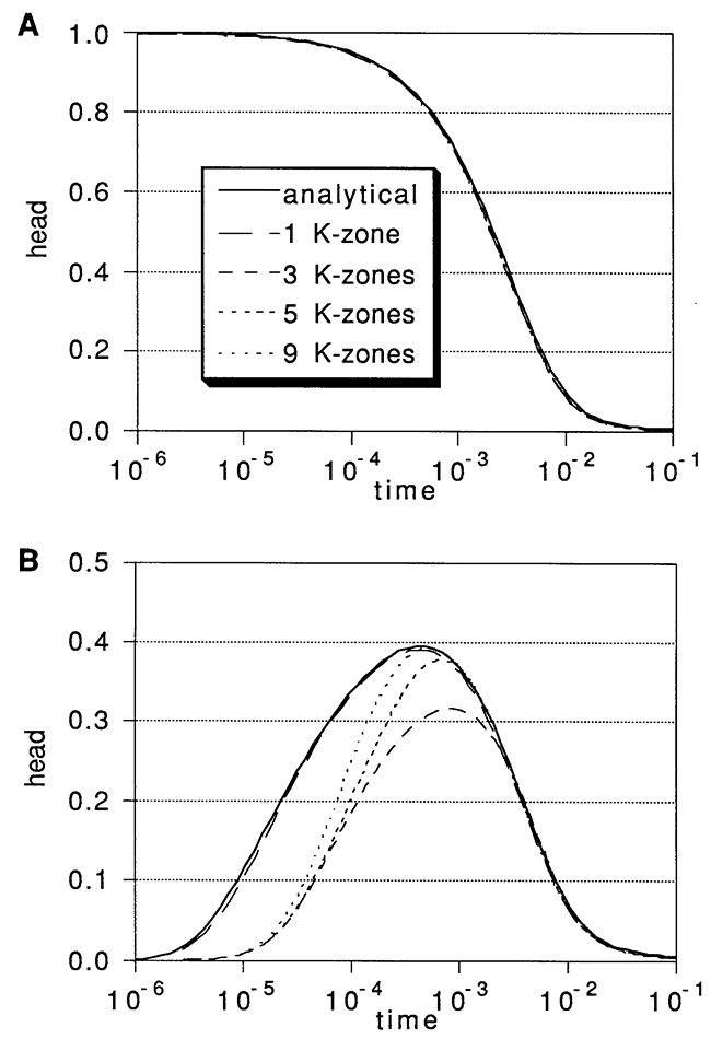
Figure 3--Layering schemes employed for results shown in Figure 2. Low and high hydraulic conductivities are those for the layered, anisotropic aquifer.
As demonstrated in Figure 2A, the numerically simulated results at the slugged well are essentially identical in the uniform case and all three layered cases. Together, they all fall just slightly below the analytical solution, as a result of discretization error. Clearly, slug tests in fully penetrating wells can provide little information about vertical variations in conductivity when the slugged well is the location of measurement. In this case the apparent hydraulic conductivity will be a thickness-weighted average of the horizontal conductivities of the layers. Figure 2B shows the responses at an observation well in the same set of fully penetrating slug test simulations. The observation point is node number 13 (the middle of the aquifer) at a radial distance of 3.7 units from the center of the slugged well. Note that even though the observation well occurs in a low-K zone in all three layering schemes, the observation well responses are different in all three cases. Thus, the results at the observation well are sensitive not only to the local properties, but also to the nearby variations in K. This demonstrates the potential contribution of observation wells to identifying conductivity variations using fully penetrating slug tests.
Multilevel slug tests (Melville et al., 1991) offer another approach for gaining more information about these vertical variations. The remainder of this paper deals with analyses of simulated multilevel slug tests performed in the four hypothetical aquifers described in Section II.
Figure 4 presents the results of a series of runs demonstrating the effects of the slugged interval length on slug-test results in the uniform aquifers (Figure 4A) and in the layered aquifers (Figure 4B) described in Section II. In these runs, the slugged interval is centered on vertical node 13 (the middle of the aquifer) and the slugged interval length increases symmetrically about that node. Results are presented in terms of the top node of the slugged interval, on the vertical axis. The hatchured area represents the top of the aquifer. To obtain each point on Figure 4, the simulated slug test results generated by the numerical model for the appropriate conditions were analyzed using the CBP solution for slug tests in fully-penetrating, finite-diameter wells. An automated well test analysis package (Bohling et al., 1990) was used to determine the best-fit Kr using nonlinear least squares. The resulting value can only be considered an apparent Kr, however, since the true flow field contains significant vertical components, while the analytical solution assumes strictly horizontal flow. Results in Figure 4 are presented in terms of a ratio of apparent Kr to true Kr, so that uniform and layered cases may be readily compared. Note that the true Kr is taken to be the thickness-weighted average of the model Kr values over the length of the slugged interval.
Figure 4--Effects of slugged interval length in the uniform (A) and the layered (B) aquifers. Slugged interval is centered at vertical node 13 and its length increases symmetrically up to the full thickness of the aquifer (25 nodes). Note that the K-configurations are also symmetric about node 13.
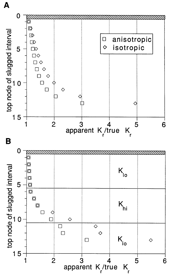
Figure 4 clearly demonstrates that the analysis of partially penetrating slug tests under the assumption of negligible vertical flow can result in a significant overestimation of the horizontal hydraulic conductivity. The vertical components of flow allow the pulse of water from the well to be dissipated more rapidly than it would be under purely horizontal flow conditions. Figure 4 also demonstrates that the apparent Kr approaches the thickness-weighted average of the true Kr values as the length of the slugged interval approaches the thickness of the aquifer. However, there is a slight discrepancy between the true and apparent values even for the fully-penetrating case. Additional test runs have shown that this difference is due to discretization error resulting from the fairly coarse discretization of the numerical model in the radial direction.
Overestimation of Kr is worse under isotropic conditions than under anisotropic conditions. As the ratio of vertical to horizontal conductivity decreases, flow is increasingly constrained to the horizontal plane.
Boundary effects are demonstrated in Figure 5. A number of runs using a three-node slugged interval (Figure SA) and a one-node slugged interval (Figure 5B) were conducted in the uniform aquifers, with the center node of the slugged interval moving from node 2 (in the three-node slugged interval case) or node 1 (in the one-node interval case) to node 13. The overall difference in apparent Kr between the two plots is a result of the increased significance of vertical flow in the one-node interval case as opposed to the three-node interval case. The boundary effects are fairly similar in both cases, although somewhat more pronounced in the one-node interval case. As the slugged interval approaches the boundary, the flow is constrained to be more horizontal, resulting in a smaller overestimation of Kr.
Figure 5--Boundary effects in the uniform aquifers using (A) a three-node slugged interval and (B) a one-node slugged interval.
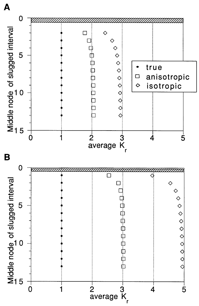
Figure 6 presents the results of CBP analyses of multilevel slug tests performed in the layered aquifers using a three-node slugged interval (Figure 6A) and a one-node slugged interval (Figure 6B). Again, results are presented as a ratio of apparent to true Kr, where true Kr is the thickness weighted average of the Kr values over the length of the slugged interval. Note that, as seen earlier, a greater overestimation of Kr occurs in the isotropic case than in the anisotropic case. Although use of a one-node slugged interval results in a greater overestimation of Kr, it does allow for clearer definition of the boundaries between contrasting conductivity values. It is reasonable to assume that analyzing the slug test data with a more appropriate model--one that accounts for partial penetration--would reduce or remove the problem of overestimation due to neglect of the vertical components of flow. In this case, it is expected that the shorter slugged interval would be the most effective for identifying the vertical variation of the conductivity values.
Figure 6--Results of CBP analyses of multilevel slug test results using (A) a three-node slugged interval and (B) a one-node slugged interval in the layered aquifers.
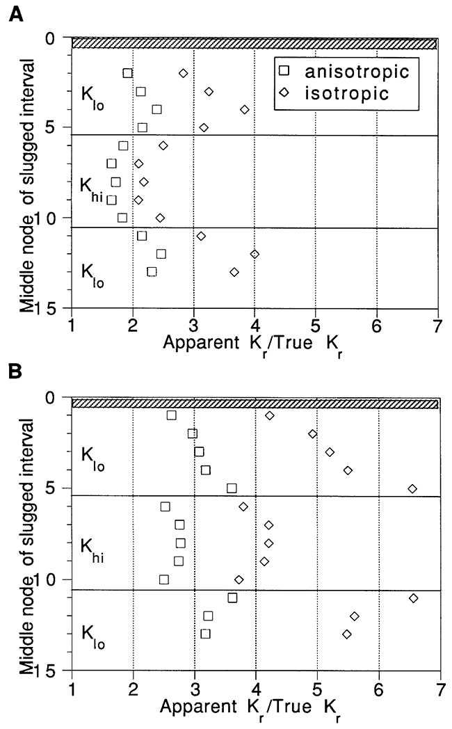
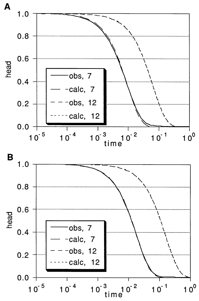
Figure 7 presents the observed and best-fit head values (from CBP analyses) for four of the runs included in Figure 6. Figure 7 A shows the results for a three-node slugged interval centered at nodes 7 and 12 in the layered, anisotropic aquifer; Figure 7B shows the results for a one-node slugged interval at the same nodes in the same aquifer. The CBP-predicted heads consistently fall below the observed heads earlier in the test, and above the observed heads later in the test. This systematic lack-of-fit is the result of neglecting the significant vertical components of flow. Unfortunately, a very similar lack of fit results from the presence of a positive well skin (low conductivity zone near the well) in a homogeneous aquifer (McElwee et al., 1990). Thus, skin effects and the effects of partial penetration may be difficult to discriminate from each other in practice.
Figure 7--Observed (obs) and calculated (calc) heads from CBP analyses of synthetic slug tests at vertical nodes 7 and 12 of layered, anisotropic aquifer using (A) a three-node slugged interval and (B) a one-node slugged interval.
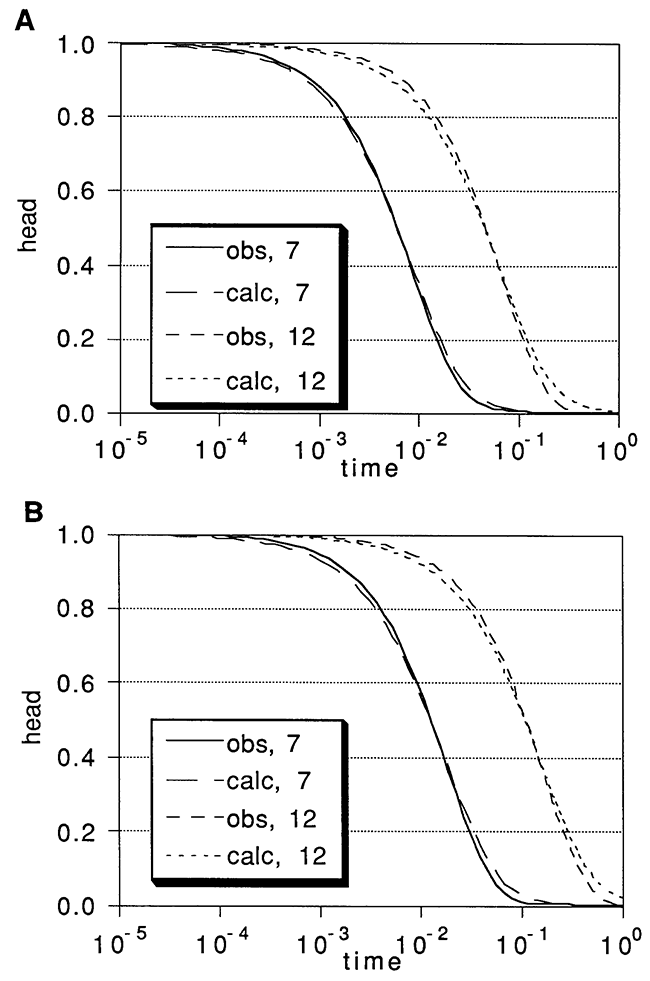
Figure 8--Results of Hvorslev analyses of multilevel slug tests in the layered, anisotropic aquifer using (A) a three-node slugged interval and (B) a one-node slugged interval in the layered aquifers and using three different assumed values of anisotropy ratio. True value of Kr/Kv is 10.
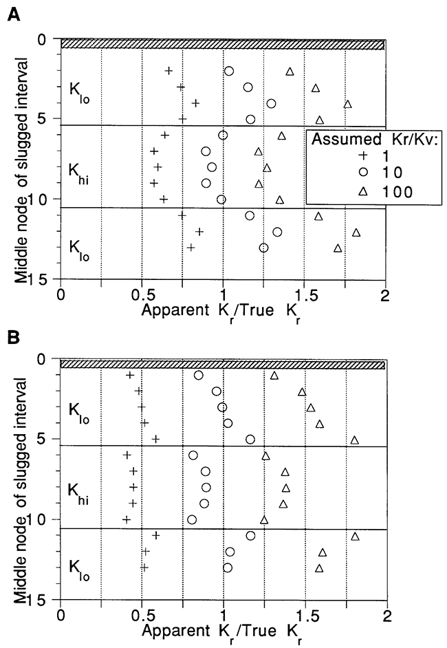
Figure 9 displays the Hvorslev model fits for the same test points as shown in Figure 7 for the CBP analyses. The results shown are for the case in which the true anisotropy ratio was used. However, the fitted results would be essentially identical for all values of anisotropy ratio, due to the perfect correlation between the model parameters. Specifying a different anisotropy ratio would result in the same optimal fit (measured in terms of the sum of squared head deviations) for a different value of radial hydraulic conductivity. Comparing Figures 8 and 9 to Figures 6 and 7 reveals that, in this case, use of the Hvorslev function improves the estimates of the radial conductivity values and provides a better fit to the observed data. This is due to the fact that the Hvorslev analyses take into account the vertical component of flow which the CBP analyses neglect. However, the Hvorslev equation must be used with caution, due to its neglect of storage effects on slug test responses (Chirlin, 1989) and its poor performance in the presence of a well skin (McElwee et al., 1990). Work is continuing on incorporating a more complete and physically correct model for partially penetrating slug tests in vertically bounded aquifers into SUPRPUMP, the nonlinear regression program (Bohling et al., 1990).
Figure 9--Observed (obs) and calculated (calc) heads from Hvorslev analyses of synthetic slug tests at vertical nodes 7 and 12 of the layered, anisotropic aquifer using (A) a three-node slugged interval and (B) a one-node slugged interval.
This presentation has demonstrated two ways in which slug tests can help to define vertical variations in hydraulic conductivity. Although analysis of the response at a fully penetrating slugged well does not yield useful information for this purpose, the responses at a number of observation wells at different vertical locations and radii will reflect the conductivity variations. In the absence of a well skin, responses measured in a fully penetrating slugged well will reflect the thickness-weighted average of the horizontal hydraulic conductivities of the layers in a perfectly stratified, confined aquifer. The following conclusions concerning the analysis of multilevel slug tests can be made: 1) Analysis of multilevel slug test results with the Cooper-Bredehoeft-Papadopulos solution can lead to a considerable overestimation of the radial hydraulic conductivity and also results in a systematic lack of fit between predicted and observed responses. 2) In these case studies, Hvorslev analyses of the multilevel slug tests resulted in better parameter estimates and less systematic lack of fit. 3) Both analysis techniques can be used to help define the effects of horizontal layering of conductivity values, with a smaller slugged interval giving better definition of layer boundaries. Work is continuing on the development of a computationally efficient analytical solution describing a fairly general slug test configuration (partially penetrating with a well skin, McElwee et al., 1990) that could be incorporated into SUPRPUMP, an automated parameter estimation program.
This research was sponsored in part by the Air Force Office of Scientific Research, Air Force Systems Command, USAF, under grant or cooperative agreement number, AFOSR 91-0298. This research was also supported in part by the U.S. Geological Survey (USGS), Department of the Interior, under USGS award number 14-08-0001-G2093. The views and conclusions contained in this document are those of the authors and should not be interpreted as necessarily representing the official policies, either expressed or implied, of the U.S. Government. The US Government is authorized to reproduce and distribute reprints for Governmental purposes notwithstanding any copyright notation thereon.
Bohling, G. c., C. D. McElwee, J. J. Butler, Jr., and W. Z. Liu, 1990, User's guide to well test design and analysis with SUPRPUMP Version 1.0: Kansas Geological Survey, Computer Program Series 90-3, 95 pp.
Butler, J. J., Jr., 1986, Pumping tests in nonuniform aquifers: A deterministic/stochastic analysis: Ph.D. dissertation, Stanford Univ., 220 pp.
Chirlin, G. R., 1989, A critique of the Hvorslev method for slug test analysis: The fully penetrating well: Ground Water Monitoring Review, v. 9, no. 2 (Spring 1989), pp. 130-138.
Cooper, H. H., Jr., J. D. Bredehoeft, and I. S. Papadopulos, 1967, Response of a finite-diameter well to an instantaneous charge of water: Water Resources Research, v. 3, no. 1, pp. 263-269.
Hvorslev, M. J., 1951, Time lag and soil permeability in ground-water observations: Waterways Exper. Sta., U.S. Army Corps of Engrs., Bull. No. 36, pp. 1-50.
Liu, W. Z., and J. J. Butler, Jr., 1992, A three-dimensional finite difference model for simulating well tests in heterogeneous aquifers: Kansas Geological Survey, Open File Report (in preparation).
Liu, W. Z, and J. J. Butler, Jr., 1991, A time-continuous finite difference approach for flow and transport simulations: Kansas Geological Survey Open File Report 91-20, 23 p.
McElwee, C. D., J. J. Butler, Jr., W. Z. Liu, and G. C. Bohling, 1990, Effects of partial penetration, anisotropy, boundaries and well skin on slug tests: Kansas Geological Survey, Open File Report 90-13, 30 p.
Melville, J. G., F. J. Molz, O. Güven, and M. A. Widdowson, 1991, Multilevel slug tests with comparisons to tracer data: Ground Water, v. 29, no. 6, pp. 897-907.
Rushton, K. R, and Y. K. Chan, 1977, Numerical pumping test analysis in unconfined aquifers: J. of Irrigation and Drainage Div., ASCE, v. 103, no. IR1, pp. 1-12.
Kansas Geological Survey, Geohydrology
Placed online Dec. 19, 2014; originally released Dec. 1991
Comments to webadmin@kgs.ku.edu
The URL for this page is http://www.kgs.ku.edu/Hydro/Publications/1991/OFR91_62/index.html