Kansas Geological Survey, Open-file Report 91-1c
Next page--Appendices
KGS Open File Report 91-1c
The objective of this pumping test was to estimate the hydraulic conductivity and storativity of a sandstone and the leakance of its overlying mudstone confining layer in the Dakota aquifer at a site in Washington County, Kansas. Prior to this test little was known about the hydraulic properties of the Dakota aquifer in this area although it is an important source of water. The test was performed near Clifton in August 1990 using a high-yield irrigation well and an observation well drilled by the Kansas Geological Survey.
Drawdown in the observation well was recorded during pumping of the irrigation well. It was then adjusted to compensate for (1) atmospheric pressure fluctuations, (2) recovery of the water level from a previous period of pumping and (3) interference from another pumping well. From water level fluctuations due to atmospheric pressure changes it was found that the barometric efficiency of the aquifer at this location is 95%, which implies its structure is very rigid. The first 27 hours of the compensated drawdown-time curve was fitted to the Hantush-Jacob leaky artesian well function by a computer program using non-linear regression. The average hydraulic conductivity and storativity of the sandstone and the leakance from the upper confining layer were calculated from this period of drawdown to be 570 gpd/sq.ft., 1.28x10⁻⁴, and 3.8x10⁻⁸ min-1, respectively. Later drawdown was greater than expected probably due to decreasing aquifer transmissivity, caused by thinning of the sandstone away from the test site rather than an abrupt no-flow boundary.
[The entire report is available as an Acrtobat PDF file (500kB).]
Pumping tests using observation wells provide invaluable information concerning the transmissivity and storage of an aquifer. They can also be used to estimate the leakage from less permeable sediments which confine the aquifer.
The Dakota aquifer is the second most geographically extensive aquifer system in Kansas. Although aquifer properties have been determined in a few areas of southwestern Kansas by means of pumping tests, there is no published record of any pumping test using observation wells in north-central Kansas. Therefore, little is known about the hydraulic properties of the aquifer in this part of the state.
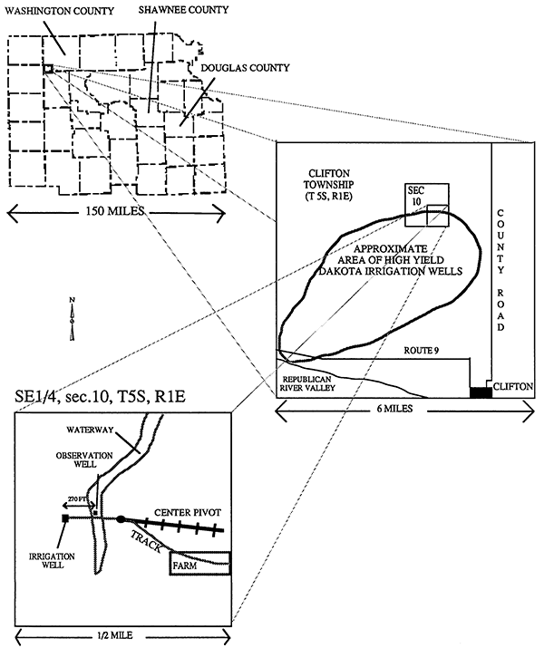
The purpose of this report is to describe a pumping test in a sandstone of the Dakota aquifer in north-central Kansas (Figure 1) in August 1990. The test was performed by pumping a high-yield irrigation well at a constant rate and observing drawdown in a nearby observation well. The drawdown was corrected by compensating for the effects of well interference, atmospheric pressure changes, and continuing recovery of the water level from a previous period of pumping. The compensated drawdown was then used to determine the transmissivity and storativity of the aquifer and the degree of leakage of water from the confining layers. The drawdown data are tabulated and plotted in appendix 4 and Figure 9 respectively.
Figure 1--Location of pumping test site in SE sec. 10, T. 5 S., R. 1 E., Washington County.
The Dakota aquifer consists of interbedded sandstones and mudstones deposited in fluvial, deltaic, and nearshore marine systems during the early Cretaceous Period (Macfarlane, Whittemore et al., 1991, p. 9). The Dakota Formation is the main geologic unit of the aquifer in Kansas, although the Kiowa Formation and Cheyenne Sandstone are also important components of the aquifer throughout much of the state.
Most of the sediments of the aquifer are fluvial system deposits; sandstones accumulated in active river channels and mudstones were deposited on floodplains and, to a minor extent, in abandoned channels. The resulting sedimentary architecture is complicated; sandstone bodies interbedded within mudstone are not in horizontal sheets. On the contrary the sandstone typically occurs in a belt-like pattern, concentrated in irregular lenses which differ in thickness, aerial extent and the degree with which they interconnect.
In 1989 and 1990, nine test holes were drilled in Washington, Republic, and Cloud counties northeast of the Republican River valley (Figure 2) to aid in understanding the sedimentary architecture of the aquifer in this area. The legal locations of the test holes and lease names are listed in Table 1.
Figure 2--Location of nine test holes in north-central Kansas drilled byu the KGS in 1989 and 1990.
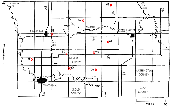
Table 1--Test holes drilled by the KGS in Republic, Washington, and Cloud counties between fall 1989 and fall 1990.
| Hole Numbera | Date Drilled | Lease Name | Location |
|---|---|---|---|
| R1 | 9/89 | Kenyon | Sec. 24, T. 4 S., R. 4 W. |
| W2 | 11/89 | Gaydusek | Sec. 10, T. 1 S., R. 2 E. |
| R3 | 4/90 | Popelka | Sec. 6, T. 3 S., R. 2 W. |
| W4 | 4/90 | Peterson | Sec. 10, T. 4 S., R. 1 E. |
| R5 | 4/90 | Benyshek | Sec. 12, T. 4 S., R. 2 W. |
| R6 | 4/90 | Cromwell | Sec. 12, T. 2 S., R. 1 W. |
| W7 | 5/90 | Leiszler | Sec. 10, T. 5 S., R. 1 E. |
| W8 | 5/90 | Nanninga | Sec. 16, T. 3 S., R. 2 E. |
| C9 | 9/90 | Feight | Sec. 7, T. 5 S., R. 1 W. |
| a. R indicates Republic County, W indicates Washington County and C indicates Cloud County | |||
Cores were taken from Rl and W2 (Figure 2) and borehole geophysical logs were obtained from these test holes. This information was used to determine the detailed characteristics of the geologic framework of the aquifer, to correlate sequences of rocks between R1 and W2, and to infer the environments in which the sediments were deposited. (Macfarlane, Wade et al., 1991). Seven other test holes were drilled and logged geophysically to determine the exact depth of changes in lithology; core samples were not obtained from these test holes. A monitoring well was installed in hole W7 and this was used as the observation well (O.1) in the pumping test.
The results of the drilling were correlated among all of the test holes. Figure 3b is a 'fence diagram' showing the correlations made between the holes in the vicinity of the pumping-test site. The true dip of the formations is not depicted in Figure 3b. In reality, the base of the Dakota Formation dips to the west-northwest at approximately 10 ft/mi, The Kiowa Formation pinches out toward the east and is not present at the site of the pumping test (Figure 3b). The Cheyenne Sandstone, which constitutes part of the aquifer in much of the southern part of the state, is not present in north-central Kansas.
Figure 3--Test holes drilled by the KGS in the vicinity of the pumping test site. The observation well used in the pumping test (O.1) was constructed in test hole W7. (a) Test hole locations. (b) Fence diagram showing the gamma ray logs of the test holes. The logs are a measure of the natural gamma radiation of the rocks penetrated by the borehole. This is an approximation of the clay content; more clayey rocks (mudstone and shale) plot to the right and less clayey rocks (sandstone and limestone) plot to the left.
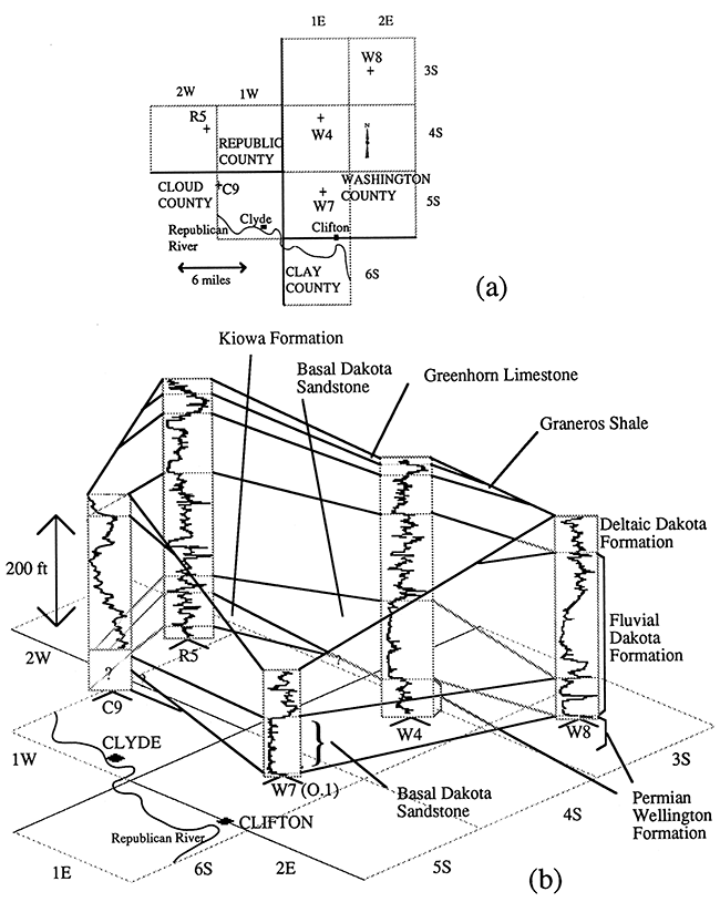
A sandstone is present at the base of the Dakota Formation in all the test holes except C9, which did not penetrate the entire thickness of the formation. Although this basal sandstone is laterally continuous throughout the area, its thickness is highly variable, and ranges from 20 to 145 ft in a horizontal distance of 11 miles between holes W4 and R5 (Figure 3). (The upper part of this channel sandstone appears to be very muddy in the gamma log of hole R5 (Figure 3b) probably due to the presence of mud rip-up clasts.)
A laterally continuous broad body of sandstone seems an unlikely product of the fluvial system described above in which the dominant lithology is overbank mudstone. However, the first sediments of the Dakota Formation in this area were deposited by relatively high-energy, high-competence streams immediately following a period of erosion when the space available for sediment accumulation was low due to a drop in sea level. This resulted in much reworking of the first Dakota Formation sediments and there was therefore little preservation of low-energy overbank mudstone and a high degree of interconnection between different channel sandstones. The basal sandstone is likely to be thickest in paleovalleys cut into the Permian and Kiowa surface by the Dakota streams and at locations where stream channels later stacked on top of one another as the depositional slope lessened and overbank mudstone began to be preserved between the channels.
The sandstones of the Dakota aquifer generally yield significant water to wells, in contrast to the mudstones which have very low permeabilities and therefore act as aquitards. The amount of water a sandstone can yield depends on its continuous areal extent and thickness as well as its grain size and degree of cementation. The good lateral continuity of the basal sandstone is therefore very important to the flow of ground water in the lower part of the Dakota aquifer.
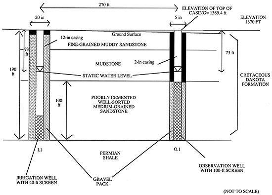
The site of the pumping test is in the outcrop belt of the Dakota Formation where erosion has reduced the thickness of the aquifer to less than 200 ft (Figure 3b, Figure 4). The sandstone in which the wells are screened is medium grained, well sorted, and poorly cemented, which is typical of the sandstone at the base of the Dakota Formation in north-central Kansas. However, its thickness of 100 ft is quite unusual. This great thickness of saturated sandstone at such a shallow depth is the main reason why irrigation wells are concentrated in this township, particularly to the southwest of the pumping test site (Figure 1). The sandstone is confined by Dakota mudstone above and Permian shale below. The difference in hydraulic conductivity between the sandstone and its confining beds was anticipated to be many orders of magnitude, and leakage effects on drawdown during the pumping test were expected to be low.
Figure 4--Cross section of the aquifer and the irrigation and observation wells.
The observation well, O.1, was drilled by the Kansas Geological Survey in May 1990. It was located 270 ft from a high-yield center-pivot irrigation well, henceforth referred to as I.1, on the edge of a waterway near the center of SE Sec. 10, T. 5 S, R. 1 E near Clifton, southwestern Washington County (Figure 1). Optimum distance between O.1 and I.1 was determined from expected drawdown based on estimates of aquifer transmissivity as well as on practicalities such as site access, position of underground pipe and cable, and location of the waterway.
A 5-in hole was drilled using mud rotary with a drag bit to a depth of 191 ft. The hole was then logged using gamma ray, spontaneous potential, resistivity, and caliper measuring tools. The gamma ray log of the hole is shown in Figure 3b. This information was used to determine the exact depth to the top and base of the sandstone aquifer. O.1 was then constructed as shown in Figure 4; it was screened and gravel packed throughout the sandstone to insure no vertical flow effects during a pumping test. The total length of screen used was 100 ft. Immediately above the screen and gravel pack, the borehole was sealed with 7 ft of bentonite chips. The uppermost 75 ft of hole was filled with a mixture of bentonite chips and shale which had sluffed off into the hole overnight. The hole was plugged at the top with bentonite chips and finally a steel cover was cemented into the ground over the PVC casing.
The well was developed using compressed air later in the month to remove accumulated fluids, mud, and cuttings. The air line was lowered to the bottom of the well and air was forced through it using a compressor. This lifted water from the well at a rate of approximately 20 GPM. The well was developed for three hours in this way until there was no trace of drilling mud in the water.
(a) On July 2, 1990, two transducers were set in O.1 at a depth of 95 ft below the top of the casing, i.e. 22.4 ft below the May static water-level. The transducers were designed for a pressure range of 10 psi which is equivalent to 23 ft of water. These transducers were connected to a Hermit Data Logger which was programmed to record the depth to water to the nearest .01 ft from the top of the casing every hour. Two transducers were used rather than one in order to insure consistency of measurements and to insure that data were not lost due to a transducer malfunctioning. This precaution proved to be worthwhile later in July when one of the transducers ceased to function. The water-level monitoring station was protected with a weatherproof, insulated cover.
(b) On the same day a barograph was located 1/4 mile from the well in a farm building and calibrated by the atmospheric pressure at the local weather station in Concordia. This instrument recorded the atmospheric pressure for the rest of the summer on paper charts. According to manufacturers specifications, the barograph had an accuracy of ±O.15 mb and a resolution of 0.2 mb. The accuracy and resolution of this instrument were insured by periodically comparing its reading to the local weather station reading at various pressures.
(c) On July 12, a McCrometer bolt-on saddle, propellor-driven flow meter was fitted onto the irrigation well. This device indicates the flow rate using an odometer which displays total gallons pumped as well as current pumping rate. To insure straight, laminar flow and accuracy of the meter, the manufacturer recommends a minimum of 8 inches of straight pipe downstream from the meter and 40 inches upstream. The length of straight, constant-diameter pipe leading from the well was limited so the meter was installed with 8.5 inches of straight pipe downstream and 35.5 inches upstream. Straightening vanes were therefore also installed immediately upstream from the meter.
The meter was calibrated for a pipe with an internal diameter of 7.872 in. (internal radius 0.328 ft), The actual internal diameter of the pipe, measured during installation of the meter, is 8.24 in.; its radius is 0.343 ft. Flow rate through a pipe is proportional to the square of its internal radius (IR2). The IR2 of the pipe is 9.6% greater than the IR2 the meter was calibrated for. Flow meter readings were therefore corrected by multiplying by a factor of 1.096.
Before the pumping test began on August 7, data were collected from the monitoring equipment described above for 4 weeks. I.1 was in use for most of the first 11 days of this period, through to July 21. Between 04:00 hrs, July 21 and 14:36 hrs, August 7, I.1 was not pumped due to wet weather. From July 22 to August 6 none of the other irrigation wells in the field to the southwest were pumped either. This allowed the aquifer to recover to within 3 ft of its pre-irrigation season level from a maximum drawdown of close to 16 ft.
The water-level data were downloaded from the datalogger directly onto a microcomputer at the Kansas Geological Survey. Atmospheric pressure data in millibars were entered into the microcomputer at the keyboard and converted into feet of water. These data were used
Depths to water and atmospheric pressure fluctuations from the first week of August were also used to quantify the effects of (a) aquifer barometric efficiency and recovery; and (b) well interference from another irrigation well which began pumping on August 6. These effects were then used to adjust the raw water-level data from the observation well in order to observe fluctuations from pumping only.
Atmospheric pressure data recorded on the barograph in early August are tabulated in Appendix 1. The uncommon pressure unit 'feet of water' was used to facilitate easy comparison of the amplitudes of the atmospheric-pressure and water-level fluctuations. Water-level data from early August are tabulated in Appendix 2. Both water-level and atmospheric-pressure data were processed and analyzed using the Lotus123 and Grapher software.
At the start of August the water level in the aquifer was still recovering from the period of pumping which had ended 10 days previously. This can be seen in Figure 5, a graph of depth to water and atmospheric pressure measured between 00:00 hrs, August 1 and 09:00 hrs, August 6. The water level rose overall despite an increase in atmospheric pressure which had the effect of pushing the water level down.
Figure 5--Atmospheric pressure and depth to water (d) in O.1, early August 1990.
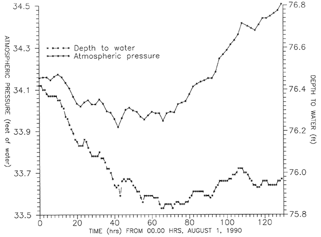
The water level of a recovering aquifer rises at a rate which decreases with time as the water level approaches its pre-pumping static level. At large time since pumping ceased, the recovery rate of an aquifer is typically inversely proportional to time and the total amount of recovery per log cycle of time is a constant. (In the same way, at large time during pumping of a well, drawdown vs. time will plot as a straight line on semilog. paper; this property is used by the Jacob StraightLine Method for solution of pumping test data.)
Two values of time were selected (0 hrs and 92 hrs in Figure 5) at which the atmospheric pressure was the same. These times correspond to 260 hrs and 352 hrs after I.1 was switched off respectively. The difference in depth to water at these times was due solely to the recovery of the aquifer because there was no difference in atmospheric pressure. The rate of recovery per log cycle of time during this period was assumed to be constant and it was determined from the slope of a straight line connecting these two points on a graph of depth to water against log time. This rate was found to be 4.0 ft per log cycle of time, which means that the water level would rise 4.0 ft during the period between 100 and 1000 hours after pumping ceased.
Recovery, R, since 00:00 hrs, August 1, could then be described in the following way:
R = 4.0 x (log (t + 260) - log 260)
where t = time (hrs) from 00:00 hrs August 1st onwards. Using this formula, when t = 0 (at 00:00 hrs, August 1), R = 0 and when t = 100 hrs (at 04:00 hrs, August 5) R = 0.57 ft.
Depths to water during the first 130 hours of August were then adjusted to mask the recovery of the aquifer in the following way:
d'=d-(-R)
(because depth to water is positive downwards and recovery is positive upwards)
i.e. d' = d + R
where
d' = depth to water (ft) compensated for aquifer recovery, and
d = depth to water (ft) recorded on the Hermit.
t, d, and d' are tabulated in Appendix 2.
Figure 6 is a plot of d' and atmospheric pressure vs. time. The variations in water level are in phase with and of similar amplitude to the variations in atmospheric pressure. The effect of an increase in atmospheric pressure is to push the water level in the well down in the same way as the water level in a manometer would be pushed down. Similarly, a decrease in atmospheric pressure causes a rise in the water level in the well. From Figure 6 it can be seen that the overall drop in atmospheric pressure during the first 40 hours of August of a little over 0.2 ft of water induced a change in water level of the same amplitude. Also, the increase in atmospheric pressure of 0.50 ft of water during the following 88 hours induced an increase in depth to water of 0.47 ft.
Figure 6--Atmospheric pressure and depth to water in O.1 compensated for aquifer recovery (d'), early August 1990.
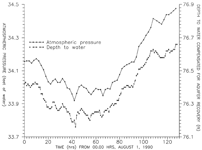
The barometric efficiency of an aquifer, BE, equals Δh/Δpa, where Δh is the change in water level in feet induced by a change in atmospheric pressure, Δpa, measured in feet of water.
Overall, Figure 6 shows that changes induced in the water level are 0.95 (±0.05) times the magnitude of changes in the pressure. This means that the barometric efficiency of the aquifer is close to 0.95 (±0.05). A barometric efficiency of this magnitude is quite exceptional and implies that its structure is very rigid and that it is well sealed off by confming sediments. The barometric efficiency of most confined aquifers is between 0.20 and 0.75 (Todd, 1967, p. 159).
Todd (1967, p. 161) gives a formula linking the barometric efficiency of an aquifer to its modulus of elasticity (Es), the porosity (α) of its structure and the bulk modulus of compression of water (Ew) which is approximately 300,000 psi.
BE = αEs / (αEs + Ew)
From this formula it can be seen that BE is close to 1 if Es » Ew.
If BE = 0.95 and the porosity, α, is estimated at approximately 30%,
0.95 = 0.3Es / (0.3Es + Ew).
It follows that Es = 63Ew, i.e. the modulus of elasticity of the structure of the aquifer is 63 times the bulk modulus of compression of water and the structure of the aquifer is therefore very rigid. This seems unlikely due to the poor lithification of the Dakota sandstone, but it may reflect high competence of the overlying confining beds and good compaction of the sandstone when it was buried by several hundred feet of sediment later in the Cretaceous Period.
Todd (1967, p. 162) also describes a way of estimating the storativity of a confined aquifer from its barometric efficiency:
Storativity, S = αγb/EwBE
where y = specific weight of water = 62.37 lbs/ft3 at 60 °F, and b = thickness of aquifer.
Using this formula,
S = (0.3 x 62.37 x 100) / (300,000 x 122 (ft2) x 0.95) = 4.6E-5.
This result is approximately 1/3 the magnitude of S determined later from the pumping test and raises questions concerning the validity of the above formulae linking barometric efficiency and storativity in a confined aquifer. However, it is beyond the scope of this report to explore this subject further. For the purpose of this pumping test it is sufficient to note that changes in atmospheric pressure induce changes in water level in the observation well of approximately the same amplitude.
At 09:36 hrs, August 6, 29 hours before the beginning of the pumping test, a second nearby irrigation well, I.2, 2200 feet to the west of I.1 was started up at an unknown pumping rate and began to affect the water level in O.1.
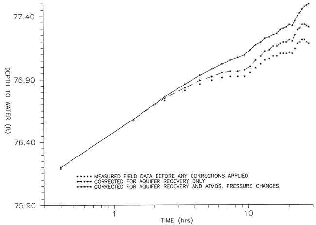
Measured drawdown due to this well was adjusted for the aquifer recovery rate of 4.0 ft per log cycle determined above. It was also adjusted for effects of atmospheric pressure changes at the rate of 0.032 ft of water level increase per millibar decrease in pressure (representing a barometric efficiency of 95% determined as described above). The effects of these adjustments on the I.2 drawdown curve are illustrated in Figure 7. The compensated drawdown due to I.2 was determined to be 0.70 (±O.5) ft per log cycle of time from this semilog plot. The measured and adjusted depths to water used in Figure 7 are tabulated in Appendix 3.
Figure 7--Drawdown due to an irrigation well, I.2, 0.42 miles from O.1.
Theis (1935) related the drawdown in an observation well to the discharge rate of water from a pumping well using aquifer properties of transmissivity and storativity:
s*= (Q/4πT) W(u)
where W(u) is the "well function," an infinite series given by
W(u) = [-.5772 - ln u + u - u2/2x2! + u3/3x3! - u4/4x4! + .... ].
The argument u is given as
u = r2S/4Tt.
In these equations, s* is the drawdown induced in the observation well at a distance, r, from the pumping well after a time, t, of pumping if the well is pumped at a constant rate, Q. T and S are the aquifer properties of transmissivity and storativity respectively.
In applying this solution, it is assumed that flow is in the range of Darcy's Law and that water is discharged instantaneously from storage in the aquifer when pumping begins. It is also assumed that the wells fully penetrate the aquifer, which has constant thickness and negligible slope and is homogeneous and isotropic.
The Theis solution does not consider the possibility of leakage of water from the confining layers above or below the aquifer. Hantush and Jacob (1954) modified the Theis solution to include consideration of leakage from a confining layer:
s*= (Q/4pT) W(u, r/B)
B is the "leakage factor," given by B = (Tb'/K')1/2,
assuming there is only one leaky confining layer,
where b' is the thickness of the confining layer, and
K' is its vertical hydraulic conductivity.
In addition to the assumptions listed above, this Hantush-Jacob solution assumes leakage through the confining layer is vertical and proportional to drawdown, the head in the deposits supplying the leakage is constant, and storage in the confining bed is negligible.
The equation is valid for all values of rs (radius of well screen), provided that
rs/B < 0.1 and t > (30rs2S{f) [1 - (10rs/b)2]
In order to determine T, S, and B using the Hantush-Jacob or Theis well functions, drawdown in an observation well should be recorded over a range of time from seconds to hours while the pumping well is discharging at a constant rate. A common method of solution facilitated by modern computing capabilities is to use non-linear regression to estimate the values of T, S, and B that produce synthetic drawdown/time data which most closely match the observed data in terms of the sum of the squared residuals. (The residual is the difference between observed and synthetic drawdown at a particular time.) This method was used to estimate aquifer properties from the pumping-test drawdowns.
Due to the water stored in a well when pumping begins, water will not be released instantaneously from storage in the aquifer and so, at early time, the Hantush-Jacob and Theis well functions are not valid. Walton (1987, p. 3) provides a formula with which to determine the critical time after which pumping well storage becomes insignificant:
ts = (5.4E5 (rw2-rc2)) / T
where ts = critical time (min),
rw = internal radius of well casing, (ft),
rc = external radius of drop pipe inside well, (ft) and
T = transmissivity of the aquifer, (gpd/ft)/
For well I.1, rw = 0.5 ft, rc = 0.25 ft and T = 57000 gpd/ft (from section 5), Therefore, using the formula above, ts = 1.8 min.
To insure no well storage effects, final values of T, S, and L were determined using only data from later than 3 minutes into the pumping test (section 5).
The pumping test itself began at 14:36 hrs, August 7th, 29.00 hours after I.2 began pumping. The irrigation well, I.1, was pumped at a rate of 592 GPM. During irrigating in July, this rate had been determined to be the normal sustainable pumping rate of the well after several hours of pumping. Initially, the pump was throttled back so as not to exceed this rate while the water level in the well was still high. Total volume pumped was read from the odometer every 5 minutes for the first 30 minutes of the test to determine the pumping rate as accurately as possible and to insure it was constant. No variation in the pumping rate was detected.
The datalogger was programmed to record depths to water to the nearest 0.01 ft at logarithmically increasing time intervals beginning at 0.2 seconds. (Drawdown was calculated to the nearest 0.01 ft for a time t after the onset of pumping by subtracting the initial depth from the depth at time t.) Pumping of I.1 was stopped after 33 hours when drawdown was nearly 9 ft and the time interval between depth measurements was 100 minutes. Eight hours later, pumping was resumed at the same rate for a further 70 hours, during which a maximum drawdown of 11.64 ft was reached. Recovery of the aquifer was then recorded for over 100 hours at a rate of one measurement every 100 minutes for the first 50 hours, dropping to one every 127 minutes for the last 50 hours.
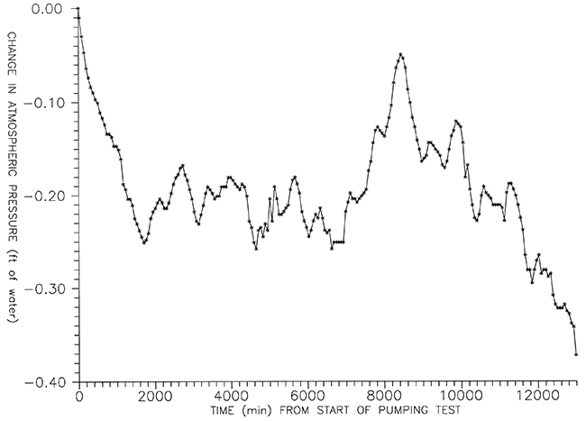
Figure 8--Change in atmospheric pressure during the pumping test.
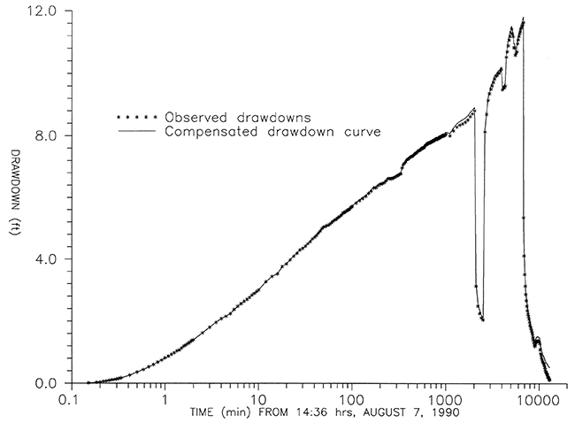
Measured depth to water, drawdown, and compensated drawdown from this nine-day period are tabulated in Appendix 4. Figure 9 shows the fully compensated and original observed drawdown plotted against logarithmic time for the complete nine days of data.
Figure 9--Observed and compensated drawdowns over the full nine days of the pumping test.
Drawdown was adjusted to compensate for the effects of overall aquifer recovery, drawdown due to I.2, and atmospheric pressure changes. These corrections are described below in section 4.3.
Measured drawdown due to pumping of I.1 was adjusted to remove the effect of I.2.
I.1 began pumping 29.0 hours after I.2 and the drawdown due to I.2 before I.1 began pumping had been determined to be 0.70 ft per log cycle of time (see section 3.3 (b), above). Assuming this rate continues to be remain constant (which is a reasonable assumption after large time), drawdown due to I.2 after I.1 began pumping can be expressed in the following way:
s (I.2) = 0.70 x (log ((t/60)+29.0)-log 29.0)
where t is time (min) since pumping of I.1 began,
log 29 is the log time at the start of pumping of I.1
and log ((t/60)+29.0) is the log time after I.1 has been pumping t minutes.
Drawdown, s' (ft), in O.1 compensated for interference from I.2 can then be expressed in the following way:
s' = s - s (I.2)
where s = drawdown (ft) in O.1 due to I.1 and I.2, calculated directly from measured depths to water. By substituting for s(I.2),
s' = s - 0.70 x (log ((t/60)+29.0)-log 29.0).
For example, at time, t = 0, s' = s = O.
After 1000 minutes of pumping of I.1 (t = 1000 min), drawdown in O.1 due to I.2 (s(I.2)) is 0.14 ft, so drawdown due to I.1 (s') is 0.14 ft less than the drawdown directly calculated from measured depth to water(s), i.e. at t=1000 min, s' = (s - 0.14) ft.
Similarly at t = 2000 min (33 1/3 hrs), s' = (s - 0.23) ft.
This well-interference adjustment decreases all drawdowns 30 minutes or more after pumping began.
Drawdown was adjusted to remove the effect of aquifer recovery, which was still occuring at a rate of approximately 0.1 ft/day, 17 days after I.1 was last pumped.
The pumping test began 418.6 hours after I.1 was last pumped. The recovery rate per log cycle of time had been determined to be 4.0 ft per log cycle of time between 260 and 352 hours (see section 3.3 (a), above). Assuming this rate per log cycle continues to remain constant, continuing recovery, R, during the pumping test period can be expressed in the following way:
R = 4.0 x (log ((t/60)+418.6) - log 418.6)
where t is time (min) since pumping of I.1 began,
log 418.6 is the log time since recovery began, at the start of pumping of I.1, and
log ((t/60)+418.6) is the log time since recovery began, after I.1 has been pumping t minutes.
Drawdown, s" (ft), compensated for aquifer recovery as well as interference from I.2, can then be expressed as follows:
s" = s' + R.
Substituting for R:
s" = s' + 4.0 x (log((t/60)+418.6) - log 418.6)
where t is time (min) since pumping of I.1 began.
For example, using this formula, at time, t = 0, s" = s' = s = O.
After 1000 minutes of pumping of I.1 ( t = 1000 min), recovery in O.1 since the pumping test began is 0.07 ft, so drawdown due to I.1 and compensated for recovery (s") is 0.07 ft more than the drawdown compensated for interference from 1.2 but not for recovery (s'),
i.e. at t = 1000 min, s" = (s' + 0.07) = (s - 0.07) ft.
Similarly at t = 2000 min (33 1/3 hrs), s" = (s' + 0.13) ft = (s - 0.10) ft.
This recovery adjustment had the effect of increasing all drawdowns 90 minutes or more after pumping began.
Drawdown was adjusted to remove the effect of atmospheric pressure changes.
Drawdown in O.1 due to an increase in atmospheric pressure is given by the product of the barometric efficiency and the increase in pressure measured in feet of water. The barometric efficiency of the aquifer had previously been determined to be 0.95 (see section 3.3 (a), above). Drawdown was therefore compensated for changes in atmospheric pressure using the following formula:
s* = s" - 0.95 x Δpawhere Δpa = difference (in feet of water) between the atmospheric pressure at time t and the atmospheric pressure at the start of the pumping test (Δpa is positive for increased pressure and negative for decreased pressure), and s* = drawdown (ft) compensated for aquifer recovery, interference from I.2, and atmospheric pressure changes, referred to henceforth as the "compensated drawdown."
Atmospheric pressure measurements recorded on charts during the pumping test and values of Δpa are tabulated in Appendix 5. Values of Δpa were determined for all times at which depth to water was recorded from a plot of the atmospheric pressure measurements in Appendix 5 (Figure 8).
Examples of the effect of eliminating atmospheric pressure changes during the pumping test are:
at t = 0, s*= s" = s' = s = 0
at t = 1000 min, s*= (s" + 0.14) ft = (s' + 0.21) = (s + 0.07) ft
and at t = 2000 min, s*= (s" + 0.20) ft = (s' + 0.33) ft = (s + 0.10) ft.
This pressure adjustment affects all drawdown measurements 24 minutes or more after pumping began. This is due to a sharp decrease in atmospheric pressure coinciding with the first 24 hours of the test (Figure 8). Atmospheric pressure never rose above its initial level throughout the nine days of pumping test data collection. Δpa was always negative and so all drawdowns after 24 minutes were greater once they were adjusted for the change in atmospheric pressure.
Determinations of transmissivity, storage, the leakage factor of the confining layer, and approximate boundary conditions were made from the initial period of uninterrupted pumping only, for the following reasons:
Suprpump (Bohling et al., 1990), a microcomputer software package incorporating the Hantush-Jacob and Theis well functions, was used to analyze the compensated drawdown/time data (see Methodology, above). Suprpump uses non-linear regression to estimate the well function parameters that produce synthetic drawdown/time data which most closely match the observed data in terms of the sum of the squared residuals. The solutions of the well function parameters for various intervals of time are listed in Table 2.
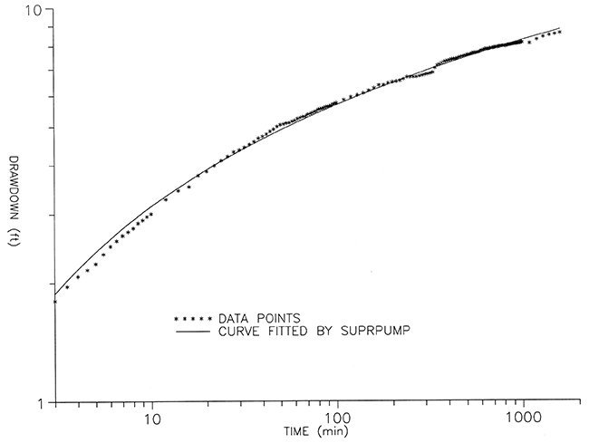
Values of transmissivity, storativity, and leakage coefficient were determined using the leaky artesian Hantush-Jacob function, the theory of which is described above under Methodology. Figure 10 shows the compensated drawdown data points and the computer-generated fitted curve for the period 3 to 1600 minutes using this function. It can be seen from the graph that the match is very good. A simple Theis analysis (Figure 11) of the same data produced a significantly poorer fit in terms of the root mean squared residuals (.08880 compared to .06566).
Figure 10--Leaky artesian analysis of compensated drawdown between 3 and 1600 minutes of pumping.
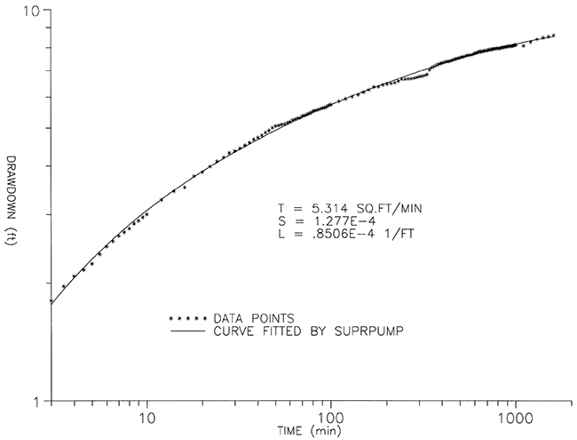
Figure 11--Theis analysis of compensated drawdown between 3 and 1600 minutes of pumping (leakage not considered).
It was found that when the data from earlier time were also considered using the Hantush-Jacob function, the difference they made to the aquifer properties was less than 3% in the case of transmissivity and storativity and less than 7% in the case of the leakage coefficient.
Figure 12 shows that the synthetic curve of Figure 10, when extended to early time, matches the early compensated drawdown surprisingly well. This is despite the expected effect of pumping well storage. If well storage was important the observed drawdowns would be expected to lie significantly below the computer generated curve at early time.
Figure 12--Compensated drawdown between 0.15 and 1600 minutes of pumping and the fitted curve from figure 10.
The best fit to the first 1600 minutes of data was obtained without simulating boundary conditions. Thus, no significant boundary effects were observed in the first 1600 minutes of data. Therefore, final estimates of aquifer parameters were made from the interval 3-1600 minutes. The best fit to the data from the interval 3-2000 minutes was obtained by including parallel no-flow boundaries at a distance of approximately 2 miles. Later drawdowns are increased significantly by boundary or aquifer thinning effects or possibly by well interference from another pumping well. This is particularly obvious (Figure 9) in the upward deviation of the drawdowns recorded later than 3000 minutes. In addition, recovery data recorded after pumping stopped are best matched with synthetic drawdowns using a lower transmissivity than during initial pumping and also simulating two barrier boundaries approximately 2 miles away.
Table 2--Values of aquifer properties determined from the pumping test. Underlined values are set as known quantities.
| Period of data considered (min) |
Transmissivity, T (ft2/min) |
Storativity, S | Leakage coefficient, L (ft-1) |
RMS res. (ft) | No-flow boundaries simulated |
|---|---|---|---|---|---|
| 3-1600 | 5.643 | 1.088E-4 | Theis; L not considered |
.08880 | NONE |
| 0-1000 | 5.368 | 1.237E-4 | .7702E-4 | .05997 | NONE |
| 0-1600 | 5.359 | 1.241E-4 | .7955E-4 | .06055 | NONE |
| 0-2000 | 5.387 | 1.229E-4 | .7245E-4 | .06224 | NONE |
| 3-1000 | 5.315 | 1.277E-4 | . 8460E-4 | .06531 | NONE |
| 3-1600 | 5.314 | 1.277E-4 | .8506E-4 | .06566 | NONE |
| 3-2000 | 5.363 | 1.249E-4 | .7510E-4 | .06789 | NONE |
| 3-2000 | 5.304 | 1.281E-4 | .8939E-4 | .06655 | 2, each 2 miles away |
| 6717-9000 | 4.510 | 1.277E-4 | .4362E-4 | .06263 | NONE |
| 6717-9000 | 4.380 | 1.277E-4 | .8073E-4 | .04261 | 2, each 2 miles away |
|
where L is the inverse of the leakage factor, i.e. L = 1/B = (K'/Tb')l/2, and RMS res. is the "root mean squared residual" or the quadratic mean difference between observed and synthetic drawdown. It is a measure of how well the synthetic drawdown fits the observed drawdown. |
|||||
These features of the later drawdown and recovery are probably due to the sandstone thinning within approximately 2 miles of the site rather than terminating abruptly. A sudden limit to the extent of the sandstone is unlikely geologically because this sandstone lies at the erosional base of the Dakota Formation which is laterally continuous in test holes in the area (Figure 3b). However, at this site the basal sandstone is exceptionally thick and a thinning of this sandstone within a few thousand feet is therefore likely. This interpretation is supported by the fact that irrigation wells in the area are not scattered universally but are concentrated to the south and west of the site, where the yield is highest, implying that the sandstone thins toward the north and east.
From the data collected between 3 and 1600 minutes,
T = 5.3(±0.3) ft2/min = 7600 (±400) ft2/day
S = 1.28(±0.06)x10-4
L = 0.85(±0.08)x10-4 ft-1
The Hantush-Jacob conditions that rs/B < 0.1 and t > (3Ors2S/T) [1 - (10rs/b)2] were both satisfied for all values of t at which drawdowns were measured.
From L = 1/B = (k'/Tb')l/2, 'leakance', k'/b', = L2T = 3.8(±0.6)x10-8 min-1.
Estimated saturated thickness of mudstone above sandstone aquifer, b' = 40 (±5) ft. (Although hydraulic head in the aquifer before irrigation season was only 15 ft above the top of the aquifer, it is likely that the mudstone above that level is very nearly if not completely saturated.)
Therefore, vertical hydraulic conductivity of confining layer, k'= 1.5 (±0.4)x10-6 ft/min = 2.2 (±O.6)x10-3 ft/day ( = 0.81 (±0.22) ft/yr)
= 0.016(±0.004)gal/day/ft2 (= 6.0(±1.6) gal/yr/ft2).
If the saturated thickness of the confining layer is only 18(±3) ft, vertical hydraulic conductivity of the confining layer,
k' = 6.9(±2.1)x10-7 ft/min = 9.9(±3.0)x10-4 ft/day (= 0.36(±0.12)ft/yr),
= 7.4(±2.2)x10-3 gal/day/ft2 (= 2.7(±0.8) gal/yr/ft2).
Both of these are reasonable results within the range expected of a clay-rich mudstone.
As is often the case in pumping tests, the main source of error in this test is likely to be in the value of the pumping rate. During the first 30 minutes of pumping, in which the pumping rate was determined every five minutes, there was no detectable variation in the rate. However, for the rest of the test the pumping rate was not observed. In theory, in a homogeneous aquifer, the Jacob sernilog plot in Figure 9 should follow a straight line after the initial curve at early time but slight deviations from a straight line can be seen in this graph. These changes in gradient are likely to be due to slight fluctuations in the pumping rate but may also reflect inhomogeneities in the aquifer.
Two other factors contributed to error in the flow rate measurement: one was the lack of sufficient straight pipe upstream from the meter to satisfy manufacturers recommendations. Also, a correction factor had to be introduced because the meter was calibrated for a pipe of 5% smaller I.D. The correction factor was based on field measurements made of the I.D. of the pipe when it was cut open during installation of the meter.
The combined effect of these factors is that the pumping rate is not accurate to better than ± 5%, i.e. Pumping rate = 592 ± 30 GPM.
Drawdown due to another pumping well 2200 ft away was noted and corrected for (see error 4 below). Other irrigation wells between 1 and 3 miles away to the south and southwest were not pumping at the time the test was begun. If any of them had been activated during the pumping test, the effects would have probably been seen in the observation well within a few hours. Graph 4 shows there were no significant sudden increases in drawdown during the first 1600 minutes which were attributable to the onset of pumping at one of these wells.
The accuracy of each transducer was checked at various water levels during preliminary testing in July, This was done by comparing the transducer values displayed on the Hermit datalogger with measurements from an electric water level tape. It was found that one transducer was malfunctioning part of the time but the other one was consistently within 0.05 ft of the electric tape measurements. At no time during the collection of water level data did the head above the transducers exceed the range they were designed for and at no time did the water level drop below the level of the transducers. Values of depth to water used for analysis before and during the pumping test were those measured by the transducer which had proved itself to be consistently accurate. Transducer error is not therefore a significant factor in the determination of the aquifer properties.
The combined effect of atmospheric pressure fluctuations, overall aquifer recovery since it was last pumped, and well interference during the pumping test was not cumulative, i.e. they did not all alter the drawdown in the same direction. On the contrary, they cancelled each other out to some extent. In addition, their influence on drawdown was least significant at low time (and not detectable at all before 24 minutes of pumping) and most significant at high time. The early data are the most important in determining values of transmissivity (T) and storativity (S) of the aquifer. Thus, compensating for well I.2, aquifer recovery and atmospheric pressure changes did not significantly affect the values of T and S determined by analysis of the drawdown/time data. However, the leakage factor determined for the confining layer was altered by over 10% when the data were adjusted as described above. This is because leakage effects are only seen at relatively high time in a pumping test.
After adjustments were made to the drawdown data for the three external factors noted above, there was no significant influence on the water level in O.1 other than the pumping of I.1. This means that errors due to external influences on the water level can be discounted.
Suprpump calculated the 95% confidence limits of the aquifer properties it determined. These were ±1 % for transmissivity, T, ±3% for Storativity, S, and ±9% for leakage coefficient, L.
The program, Aquitest (Heidari and Hemmet, 1991), which also estimates aquifer parameters using non-linear regression, was used to check the results. The results obtained for T, S, and L were all within 0.5% of the results obtained using Suprpump.
The assumption that leakage only occured through the upper confining layer may not be true. If there was significant leakage from the Permian shale underlying the aquifer during the pumping test, the value of k' for the upper confining layer determined from L would be a low estimate of the true value.
The top of the sandstone aquifer being tested is at a depth of 85.0 ft below ground level, i.e. 87.5 ft below the top of the casing, which is the datum from which depth to water measurements were taken. At no time during the first 33 hours of the pumping test did the water level in the observation well fall below this level.
Thus, the effect of the water level falling below the top of the aquifer was not a factor in this pumping test.
I.1 is screened through the lower 40 ft of the sandstone only (Figure 2). Close to the pumping well shortly after pumping began vertical flow may be significant and this can affect the drawdown in an observation well. O.1 was therefore positioned a large distance from I.1 and was screened throughout the sandstone making the effect of the partially penetrating pumping well negligible.
Horizontal transmissivity, T = 7600 (± 400) ft2/day = 57000 (±3000) gpd/ft
Horizontal hydraulic conductivity, k = 76 (±4) ft/day = 570(±30)gal/day/ft2
This hydraulic conductivity is high for a sandstone- it is more typical of an unconsolidated sand such as Ogallala sand. This is mainly due to the general lack of cement in this sandstone. The poor lithification of the sandstone at the pumping test site is typical of the river channel sandstones of the Dakota Formation. Its grain size is also typical of a sandstone at the base of the formation but is at the high end of the range found in Dakota river channel sandstones in general. Therefore, this hydraulic conductivity can be considered a representative value for the basal sandstone of the formation although it is likely to be greater than the hydraulic conductivity of most sandstones higher in the formation.
The transmissivity, which is directly related to potential well yields, is not normally as great as determined in this test because most fluvial sandstones of the Dakota Formation, including the basal sandstone, are not as thick as the one studied in this pumping test.
Storativity, S = 1.28(±0.06)x10-4.
Thus, 1.3x10⁻⁶ ft3 (0.0012 ounces) of water is released from one cubic foot of the aquifer if the hydraulic head drops by one foot. This is the "specific storage" of the aquifer. This result, although apparently very small, is within the normal range typical of a confined aquifer. Watts (1989) estimated the specific storage of the Dakota aquifer in southwestern Kansas to be 2x10⁻⁶ ft-1,
Assuming there is no leakage from the Permian shale underlying the sandstone, the leakage coefficient, L of the upper confining layer =1/B = 0.85(±0.08)x10-4 ft-1.
For the confining layer, leakance, k'/b' = 3.8(±0.6)x10-8 min-1.
Maximum vertical hydraulic conductivity of the confining layer, assuming 40 feet of saturated mudstone immediately overlies the sandstone,
k'= 8 gallons per year per square foot = 1 ft/yr.
This means that recharge of the sandstone aquifer cannot exceed 8 gal/yr/ft2 (1 ft/yr) through the confining layer. Recharge is likely to be much less than this upper limit because most of the confining layer is probably not completely saturated with water and therefore has a lower hydraulic conductivity than this.
However, if there was any significant leakage from the underlying Permian shale during the pumping test, the maximum k' of the upper confining layer would be greater than the 1 ft/yr estimated above.
The sandstone aquifer at the site of this pumping test is 100 ft thick. Drawdown during pumping and recovery later than 1600 minutes was affected as if no-flow boundaries were present several thousand feet from the site. Recovery data recorded after pumping stopped are consistent with a lower transmissivity than during initial pumping. This is probably due to the sandstone thinning within 2 miles of the site rather than terminating abruptly. A sudden limit to the extent of the sandstone is unlikely geologically because this sandstone is the basal sandstone of the Dakota Formation, which in test holes in the area is laterally continuous although variable in thickness.
The combined effect of well interference, aquifer recovery, and atmospheric pressure changes on the drawdown during the pumping test was not cumulative. On the contrary, by chance these factors cancelled each other out to some extent; the decrease in atmospheric pressure and the continuing recovery from a previous period of pumping raised the water level whereas well interference from another pumping well lowered the water level. In addition, their influence on drawdown was least significant at low time (and not detectable at all before 24 minutes of pumping) and most significant at high time.
Thus, compensating drawdowns for the factors listed above did not significantly affect the values of T and S determined by analysis of early drawdown/time data.
However, the leakage factor determined for the confining layer was altered by over 10% when the data were adjusted as described above. This is because leakage effects are only significant at relatively high time in a pumping test.
The storativity (S) of the aquifer determined from the pumping test was three times the value of the storativity estimated from an equation linking S to the barometric efficiency of the aquifer. The barometric efficiency method is therefore not an accurate way of determining S, although it is useful in estimating its order of magnitude.
Water is currently being pumped from the Dakota aquifer in T. 5 S., R. 1 E., of southwestern Washington County at a rate of several hundred acre-feet per year. However, there has only been a slight drop in water levels in the aquifer in this township since most of the irrigation wells were constructed in the 1970s and early 1980s. Therefore the aquifer must be receiving recharge of several hundred acre feet per year. Leakage through the confining layer in this township alone could not account for all this recharge. It is likely that much of the recharge to the sandstone in southwestern Washington County originally enters the aquifer in topographically higher areas in the west-central part of the county (where ground-water usage is relatively low) and flows toward the south through interconnected sandstones, ultimately discharging into the Republican River valley aquifer.
Allen Macfarlane provided the inspiration for this project and contributed with much helpful advice from the planning stage to the writing stage.
In the field, the KGS drill crew, lead by Joe Anderson and Mel Kleinschmidt, drilled the observation well in addition to all the other test holes listed in table 1. John Healey logged the holes, fitted the flow meter to the irrigation well and developed the observation well. The pumping test could not have been performed without the preliminary work of these professionals as well as the full cooperation of landowners lim and John Leiszler.
During the analysis of the drawdown, Geoff Bohling kindly supplied customized variations of his program, Suprpump, which helped in the consideration of boundary conditions in particular.
Allen Macfarlane, Manoutch Heidari, Carl McElwee, and Janet Coleman reviewed the manuscript. I thank them for their time and their suggestions which helped improve the paper.
Thanks also to Jim Butler for many helpful discussions at the planning and analysis stages and to Manoutch Heidari for drawing attention to the consideration of pumping well storage.
Bohling, G.C., C. D. McElwee, J.J. Butler, and W. Liu, 1990, Users guide to well test design and analysis with Suprpump Version 1.0: Kansas Geological Survey Computer Program Series #93.
Hantush, M.S., and C.E. Jacob, 1954, Plane potential flow of ground-water with linear linkage: Transactions, American Geophysical Union, 35, p. 917-936
Heidari, M., and M. Hemmet, 1991, Aquitest, software to conduct automated aquifer test analysis: unpublished report.
Macfarlane, P.A., A. Wade, J.R. Doveton, and V.J. Hamilton, 1991, Revised stratigraphic interpretation and implications for pre-Graneros paleogeography from test-hole drilling in central Kansas: Kansas Geological Survey, Open-file Report 91-1A, 73 p. [available online]
Macfarlane, P.A., D.O. Whittemore, M.A. Townsend, J.J. Butler Jr., J.H Doveton, V.J. Hamilton, J. Coleman, T.M. Chu, A. Wade, and G.L. Macpherson, 1991, The Dakota Aquifer Program: Annual Report, FY90: Kansas Geological Survey Open-file Report 91-1, 42 p. [available online]
Todd, D.K., 1967, Ground Water Hydrology: John Wiley & Sons, 336 p.
Theis, C. V., 1935, The lowering of the piezometric surface and the rate and discharge of a well using ground-water storage: Transactions, American Geophysical Union, 16, p.519-524.
Watts, K.R., 1989, Potential hydrologic effects of ground-water withdrawals from the Dakota aquifer, southwestern Kansas: U.S. Geological Survey Water-Supply Paper 2304, 47 p.
Walton, W.C., 1987, Groundwater pumping tests, design and analysis: Lewis, 201 p.
Kansas Geological Survey, Geohydrology
Placed online May 13, 2013; originally released 1991
Comments to webadmin@kgs.ku.edu
The URL for this page is http://www.kgs.ku.edu/Hydro/Publications/1991/OFR91_1C/index.html