Kansas Geological Survey, Current Research in Earth Sciences, Bulletin 248, part 1
Prev Page--Study Area || Next Page--Results
![]()
![]()
![]()
Kansas Geological Survey, Current Research in Earth Sciences, Bulletin 248, part 1
Prev Page--Study Area ||
Next Page--Results
![]()
Processing and statistical analysis of Landsat TM datasets were the major methods used in this study. Other techniques included kite aerial photography (KAP), tree-ring measurements, and analysis of climatic records. These lines of evidence were compared to discover temporal relationships between forest growth, climatic events, and satellite observations.
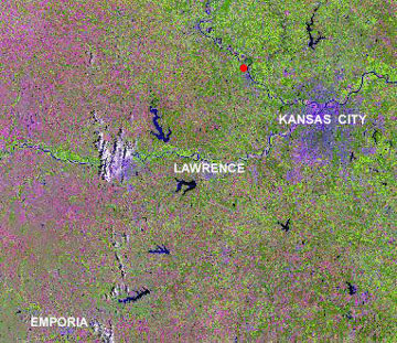
A total of eight Landsat TM datasets were obtained for the period 1987 to 1997 (table 1). To maintain the most consistent results for interannual comparison, all datasets were acquired by the Landsat 5 TM instrument, and all Landsat TM datasets were from the month of July. Use of images from the same time each year should minimize seasonal effects on vegetation phenology, soil moisture, sun angle, and other variables. During July, vegetation is in full growth, prior rainfall is generally high, and sun position is high for good illumination of the forest canopy with minimal shadows. Most images used in this study were free of clouds in the study area, except for July 1989 and, to a lesser extent, July 1992. Because of heavy cloud cover throughout the summer of 1993, it was not possible to obtain an image of the study area for July 1993. The selected scenes are from Landsat TM path 27, row 33, which includes northeastern Kansas and a small portion of northwestern Missouri (figs. 6, 7).
Table 1--Landsat 5 TM datasets selected for use in this study. Each dataset was acquired in July of the respective year.
| Scene ID | Year |
|---|---|
| LT5027033008720410 | 1987 |
| LT5027033008820710 | 1988 |
| LT5027033008920910 | 1989 |
| LT5027033009019610 | 1990 |
| LT5027033009119910 | 1991 |
| LT5027033009218610 | 1992 |
| LT5027033009419110 | 1994 |
| LT5027033009718310 | 1997 |
Figure 6--General location map for Landsat TM path 27, row 33. Map obtained from U.S. Geological Survey, EROS Data Center, Sioux Falls, South Dakota (1999).
Figure 7--Landsat TM composite browse image (23 July 1987) made from bands 3, 4, and 5, color coded as blue, green, and red. Location of the Fort Leavenworth study area indicated by red dot. Active vegetation appears in various green and yellow-green colors. Image obtained from U.S. Geological Survey, EROS Data Center, Sioux Falls, South Dakota.
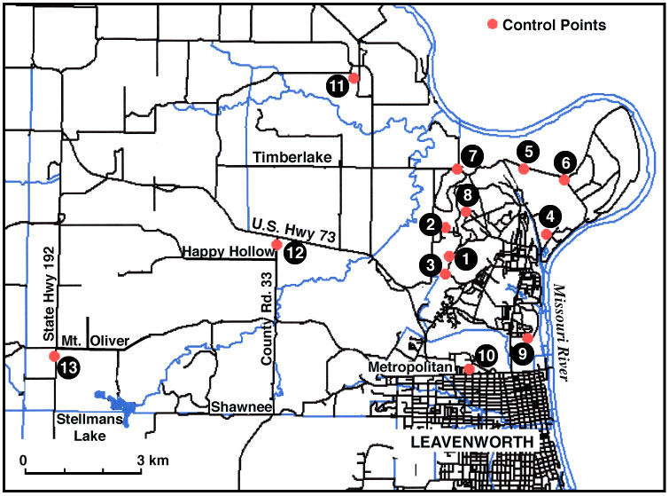
The study employed standard image-processing techniques, including haze correction, georegistration, compositing, ratioing, supervised and unsupervised classification, masking, principal-component analysis, and other operations (Avery and Berlin, 1992; Jensen, 1996). All image processing and analysis was carried out with IDRISI software. Working image windows of the Fort Leavenworth area were extracted from the full scenes using a common reference point for all datasets: an old missile base within the upland study forest (fig. 8). These windows were resampled based on ground control points within and west of the military reservation (fig. 9). For control points within the reservation, differential GPS equipment was used for field survey of UTM coordinates (Wilkins, 1997). Locations of control points to the west were derived from digital topographic maps. Resampling resulted in working images in UTM projection, zone 15, NAD27 datum. All subsequent image processing was based on these resampled windows of the Fort Leavenworth study area.
Figure 8--Landsat TM band 5 image showing old missile base in the upland study forest. This site (red pixel) was the reference point used for extracting windows from whole Landsat TM datasets.
Figure 9--Locations of ground control points used for resampling the raw Landsat TM windows. Points 1-10 were collected in the field with differential GPS equipment; points 11-13 were derived from digital topographic maps.
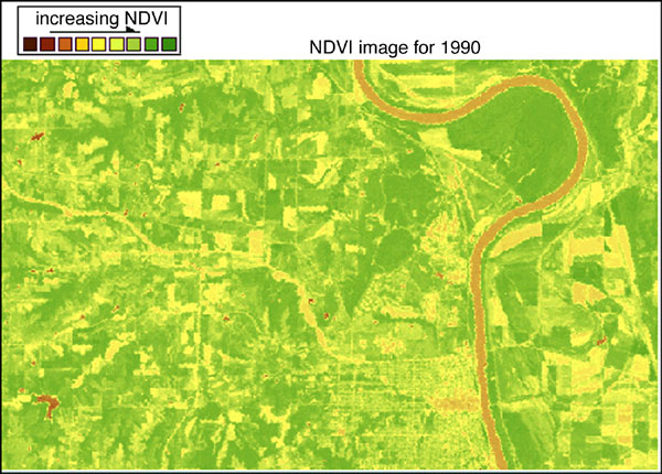
Whole-study scene NDVI values were calculated for haze-corrected windows based on Landsat TM band 4 (near infrared) and band 3 (red). Raw NDVI values are real numbers between -1 and +1. These values were expanded and converted into byte-binary format (0-255). As table 2 indicates, July 1987 had the highest NDVI value overall, and July 1990 had the lowest (figs. 10, 11). Because the 1989 dataset contained scattered clouds and cloud shadows, the NDVI value was lower than it should have been. To correct this, the clouds and shadows were isolated using unsupervised classification (ISOCLUST module). These features then were removed by creating a cloud-shadow mask, which changed slightly the overall NDVI value for July 1989 from 170.7 to 179.2 and changed its rank from 6 to 5.
Table 2--Whole-study scene NDVI values for Fort Leavenworth study area. July 1987 has the highest and July 1990 has the lowest values overall. Percentage values for each year are based on July 1987 mean NDVI value as 100%.
| Scene Date | Mean NDVI | Standard Deviation |
% | Rank |
|---|---|---|---|---|
| July 1987 | 201.1 | 28.6 | 100 | 1 |
| July 1988 | 186.9 | 33.2 | 92.9 | 4 |
| July 1989 | 179.2 | 28.7 | 89.1 | 5 |
| July 1990 | 165.7 | 26.0 | 82.4 | 8 |
| July 1991 | 173.4 | 25.0 | 86.2 | 6 |
| July 1992 | 168.8 | 22.9 | 84.0 | 7 |
| July 1994 | 190.4 | 25.0 | 94.7 | 3 |
| July 1997 | 192.7 | 26.6 | 95.8 | 2 |
Figure 10--NDVI image for July 1987 window of Fort Leavenworth study area. Green shows active vegetation, yellow is unvegetated surfaces, brown depicts water bodies and urban sites. Note contrast in greenness with fig. 11.
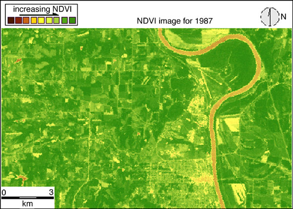
Figure 11--NDVI image for July 1990 window of Fort Leavenworth study area. Green shows active vegetation, yellow is unvegetated surfaces, brown depicts water bodies and urban sites. Note contrast in greenness with fig. 10.
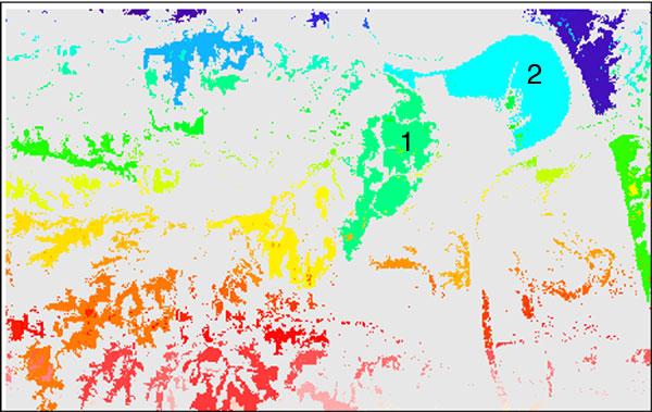
Based on its high NDVI value, the July 1987 scene was selected to represent the best development of forest canopy among the years of data. Unsupervised classification (ISOCLUST module) was carried out on the July 1987 scene to separate forest from other types of land cover. Fifteen clusters were extracted, of which two clusters (1 and 3) represented types of forest cover (fig. 12). Field checking revealed close correspondence between the forest boundaries and cluster analysis. The forest clusters were then separated, and adjacent like pixels were joined using the GROUP module (fig. 13). Polygons representing the upland and bottomland study forests were separated to create a mask for each forest. These masks were applied to the NDVI images of each year to remove all portions except for the study forests. This procedure resulted in images that portray NDVI values only for the same areas of upland or bottomland study forests. Once again, the July 1989 dataset required additional processing to remove clouds and cloud shadows from the study-forest areas.
Figure 12--Results of unsupervised isocluster classification of July 1987 Landsat TM dataset. Clusters 1 and 3 represent types of forest.
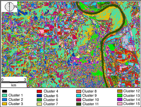
Figure 13--Forest cluster pixels grouped into polygons of contiguous pixels. Polygon 1 represents the upland study forest; polygon 2 is the bottomland study forest.
The NDVI images for upland and bottomland study forests were evaluated with principal-component analysis and image-differencing techniques. In IDRISI, the Time Series Analysis module performs principal-component analysis, which is a statistical technique for separating a multivariate dataset into uncorrelated linear combinations or components. Each component has little variance, but together they represent all the data in the original dataset. If there is significant intercorrelation within the data, the first few components account for a large part of the variance. Cloud cover and shadows in the July 1989 dataset created a problem of pixel contamination, so this dataset was omitted from the principal-component analysis. Cloud cover also affected the upland study forest for July 1992, and it was omitted as well.
Image differencing is used to detect spectral changes between two images, based on subtracting the value of cells in one image from corresponding cell values in another image. The result is an image that contains the difference values, which may be positive, zero, or negative. A histogram of difference values typically follows a symmetrical, normal distribution (Eastman et al., 1995). To determine cells of real change, a threshold is set; values beyond this threshold are considered to represent extraordinary change. Image differencing was performed for NVDI image-pairs from both upland and bottomland forests; these pairs were selected to represent change throughout the period of study: 1988-1987, 1990-1988, 1994-1991, 1997-1994, and 1997-1987. The threshold value was set in each case at two standard deviations from the mean NDVI difference.
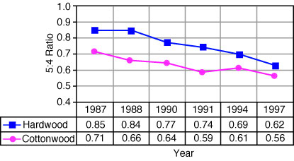
A band 5:4 ratio image was prepared for each whole July dataset to obtain the moisture stress index (MSI). (Clouds and cloud shadows were removed from the July 1989 image as noted above.) Ratios for the study forests were then extracted using the upland and bottomland forest masks derived from the July 1987 image. The results are positive real numbers in the range 0.5 to 0.9, as band 4 is generally somewhat brighter than band 5 for active vegetation. Preliminary results revealed a gradual, long-term decrease in band 5:4 ratios for both upland and bottomland study forests (fig. 14). Linear-regression analysis was used to remove the long-term downward trend from the band 5:4 ratio values. Residual values obtained from this process represent departures (positive or negative) from the trend and were used for further analysis and interpretation.
Figure 14--TM band 5:4 ratios for upland (hardwood) and bottomland (cottonwood) study forests at Fort Leavenworth, Kansas. Both forests display gradual decreases in band 5:4 ratios, though the hardwood forest ratios are consistently higher.
Climatic data for 1986 to 1997 were obtained for northeastern Kansas from the National Climatic Data Center (NCDC, 1999). Average values for temperature, precipitation, and Palmer Drought Severity Index (PDSI) were calculated for the 12-month period from July to June, preceding the July image capture date each year. For example, the average values for 1987 include the period July 1986 to June 1987. In this way, the average values indicate yearly climatic conditions leading up to the time of image capture. In addition to the 1986-1997 climatic data, older climatic data were applied to interpretation of the tree record (Nang, 1998). Similarly, field observations during the course of a winter 2000 drought were applied to the interpretation of Landsat TM imagery for the 1988-1989 drought.
Results of tree-ring analysis were obtained from Nang (1998), who collected two tree-ring cores from each of 15 oak trees in the upland forest in 1997. Sampled tree species included red oak (Quercus rubra), black oak (Q. velutina Lam.), post oak (Q. stellata Wang), white oak (Q. alba L.) and chestnut oak (Q. muehlenbergii Engelm.). Because the chestnut oak proved to have indistinct annual rings that were difficult to measure, it was not included in the analysis. Ring widths were measured for the last 30 years (1968-1997). The long-term decline in ring width, a typical tree-growth phenomenon, was removed by linear-regression analysis. The resulting residual values reflect deviations from the long-term growth trend. The residual data are reported as positive or negative values in tenths of millimeters. Annual residual values were averaged for all samples of red, black, white and post oak, the species that proved to have the most consistent records.
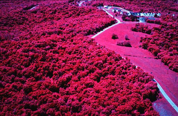
Kite aerial photography (KAP) involves the use of large kites to lift camera rigs 50-150 m (160-500 ft) above the ground. Various types of radio-controlled, single- and dual-camera systems may be employed to acquire images in visible and near-infrared portions of the spectrum (Aber et al., 1999, 2001). Beginning in 1997, KAP was employed yearly to document canopy conditions in the upland forest; the bottomland forest was photographed beginning in 1998. KAP was conducted mainly in the spring (April-June) to better understand forest greenup and to evaluate canopy structure, with and without leaves. Photographs were taken in vertical and oblique modes using color-visible and color-infrared diapositive (slide) film (figs. 15, 16). Selected photographs were scanned into digital format, with pixel resolution ranging from 10 cm to 20 cm (4 in to 8 in). The clarity of detail in such images allowed interpretation of canopy structure at submeter resolution.
Fig. 15--Normal-color kite aerial photograph of the upland study forest, Fort Leavenworth, Kansas, May 2000. Oblique view toward the south shows a fully developed forest canopy. Compare with fig. 16.
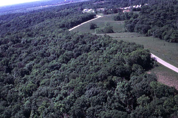
Fig. 16--Color-infrared kite aerial photograph of the upland study forest, Fort Leavenworth, Kansas, May 2000. Active vegetation appears in red and pink colors. Compare with fig. 15.
Prev Page--Study Area || Next Page--Results
Kansas Geological Survey
Web version January 25, 2002
http://www.kgs.ku.edu/Current/2002/aber/aber3.html
email:webadmin@kgs.ku.edu