Kansas Geological Survey, Current Research in Earth Sciences, Bulletin 248, part 1
Prev Page--Methodology || Next Page--Interpretation and Discussion
![]()
![]()
![]()
Kansas Geological Survey, Current Research in Earth Sciences, Bulletin 248, part 1
Prev Page--Methodology ||
Next Page--Interpretation and Discussion
![]()
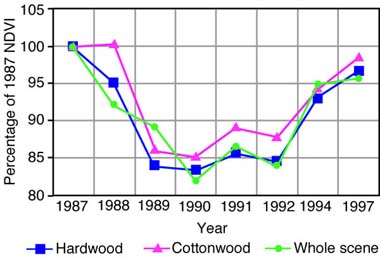
Normalized Difference Vegetation Index (NDVI) values for upland and bottomland forests are presented in table 3. The wide range in values suggests that saturation of NDVI did not take place for the study forests. The relative percentages for upland forest, bottomland forest, and whole-scene NDVI values are given in fig. 17. Percentage changes are mostly parallel, and all categories display minimum NDVI values in 1990. Contrary to the consistent overall trend, the bottomland forest shows a small increase in July 1988, and the NDVI percentages for the bottomland forest are slightly higher throughout in relation to the upland forest.
Table 3--Mean NDVI, standard deviation, and NDVI percentage values for upland (hardwood) and bottomland (cottonwood) forests. Compare with whole-study scene NDVI values (Table 2).
| Year | Hardwood Mean NDVI |
Hardwood Standard Deviation |
Hardwood % NDVI |
Cottonwood Mean NDVI |
Cottonwood Standard Deviation |
Cottonwood % NDVI |
|---|---|---|---|---|---|---|
| 1987 | 227.7 | 4.6 | 100 | 223.7 | 4.8 | 100 |
| 1988 | 216.4 | 12.2 | 95.0 | 224.3 | 6.2 | 100.3 |
| 1989 | 191.2 | 6.4 | 83.9 | 192.8 | 7.8 | 86.2 |
| 1990 | 189.8 | 7.1 | 83.3 | 190.7 | 8.3 | 85.3 |
| 1991 | 195.1 | 7.4 | 85.7 | 199.2 | 6.0 | 89.1 |
| 1992 | 192.5 | 9.8 | 84.5 | 196.4 | 4.3 | 87.8 |
| 1994 | 211.7 | 9.1 | 93.0 | 211.0 | 8.7 | 94.3 |
| 1997 | 220.0 | 7.4 | 96.6 | 220.4 | 4.8 | 98.5 |
Fig. 17--Relative NDVI values for upland (hardwood), bottomland (cottonwood), and whole-scene study areas, based on July 1987 as 100%. The lowest values in all cases are for July 1990. The bottomland forest shows an anomalous increase in July 1988.
Principal-component analysis was carried out on six-scene datasets for the upland and bottomland study forests (table 4). These results show that more than 99.9% of the variations in both study forests are accounted for by component one. This suggests that the datasets for all years are highly correlated, and this correlation is similar in nearly all respects to yearly NDVI values. Small variations are associated with components 2-6. Component 2 represents about 0.02-0.03% of the variance. This component is associated mostly with zones that are 2-3 pixels wide on edges and boundaries of both upland and bottomland forests (figs. 18, 19). The higher-order components (3-6) display even smaller values (about 0.01% or less). Such small values could be the results of slight differences in image registration or other noise effects; they are not considered significant for further interpretation.
Table 4--Percent variances for components 1-6 of six-scene datasets for upland and bottomland study forests, Fort Leavenworth, Kansas. Datasets include July forest masks for 1987, 1988, 1990, 1991, 1994, and 1997.
| Study Forest | Component 1 | Component 2 | Component 3 | Component 4 | Component 5 | Component 6 |
|---|---|---|---|---|---|---|
| Upland | 99.93196 | 0.02697 | 0.01378 | 0.01113 | 0.00914 | 0.00703 |
| Bottomland | 99.94922 | 0.01918 | 0.01312 | 0.00747 | 0.00648 | 0.00453 |
Fig. 18--Upland forest image showing component two of the NDVI principal-component analysis. Positive values indicate an increase in vegetation cover, and negative values show loss of vegetation cover. Most change (loss) is located on the outer perimeter and along roads and other clearings in the disjunct forest cover.
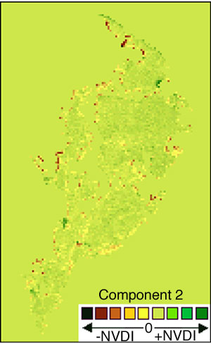
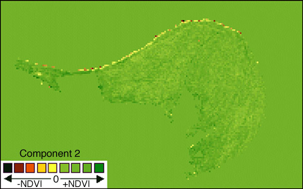
Fig. 19--Bottomland forest image showing component two of the NDVI principal component analysis. Positive values indicate an increase in vegetation cover, and negative values show loss of vegetation cover. Most change (loss) is located on the northern perimeter of the forest along the Missouri River channel.
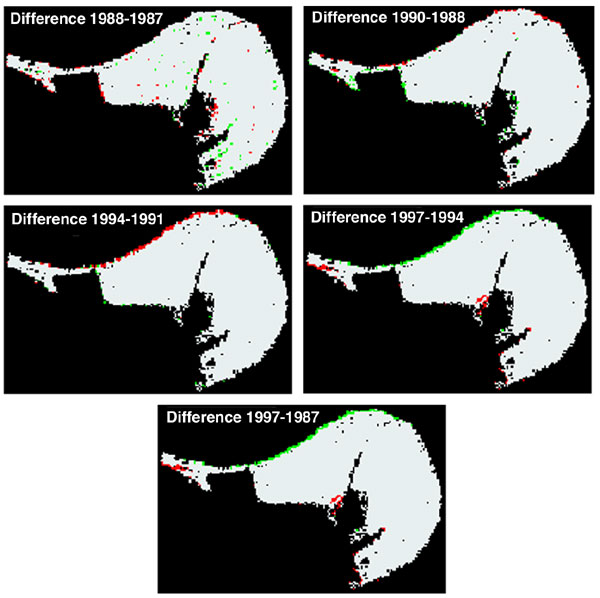
The results of image differencing for both study forests (table 5) are consistent with the trends of NDVI values and results of principal-component analysis. The most drastic declines for both forests took place during the 1988 to 1990 period (1990-1988). Once again, the bottomland study forest displays a slight increase for the period 1987 to 1988 (1988-1987), in contrast to decline for the upland study forest. The best recoveries were during the interval 1991 to 1994 (1994-1991), followed by the period 1994 to 1997 (1997-1994). The overall change from 1987 to 1997 (1997-1987) is down slightly for both study forests. NDVI difference images reveal that most changes took place around the margins of the study forests (figs. 20 and 21).
Table 5--Image differencing results for upland (hardwood) and bottomland (cottonwood) study forests, Fort Leavenworth, Kansas. Greatest declines were for 1990-1988, and best improvements for 1994-1991. Compare with fig. 17.
| Years | Hardwood NDVI Difference Mean |
Hardwood Standard Deviation |
Cottonwood NDVI Difference Mean |
Cottowood Standard Deviation |
|---|---|---|---|---|
| 1988-1987 | -6.3 | 11.0 | 0.6 | 5.6 |
| 1990-1988 | -26.6 | 10.5 | -33.5 | 8.0 |
| 1994-1991 | 16.6 | 7.1 | 11.7 | 7.2 |
| 1997-1994 | 8.4 | 6.8 | 9.4 | 7.7 |
| 1997-1987 | -2.7 | 7.3 | -3.3 | 5.3 |
Fig. 20--NDVI difference images for year-pairs of the upland study forest, Fort Leavenworth, Kansas. Most changes, both positive (green) and negative (red), are situated around the forest margin.
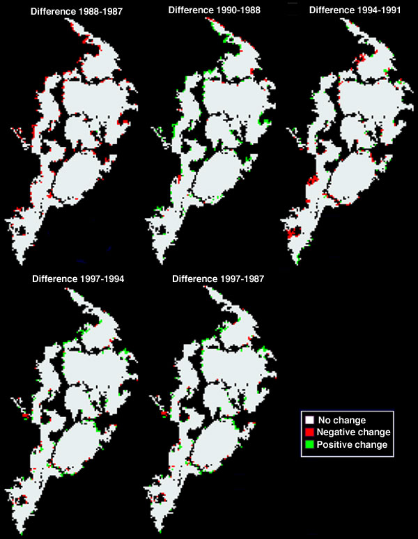
Fig. 21. NDVI difference images for year-pairs of the bottomland study forest, Fort Leavenworth, Kansas. Most changes, both positive (green) and negative (red), are situated around the forest margin.
Trend lines and residual values for TM band 5:4 ratios are presented in figs. 22 and 23 for the study forests. The trend lines display near-parallel declines with upland forest values consistently higher than bottomland forest values. Yearly increases in residual values represent leaves with lower moisture content, and decreases indicate more leaf moisture. The residual values change in similar fashion for both forests for each year except 1988, when the forests experienced opposite changes: the upland forest increased, while the bottomland forest decreased. The opposite changes in TM band 5:4 residual values for July 1988 correspond to similar anomalies in NDVI values. Both study forests experienced lowest leaf moisture (highest 5:4 residuals) in 1989 and highest leaf moisture (lowest 5:4 residuals) in 1992.
Fig. 22--Linear trends for TM band 5:4 ratios for upland (hardwood) and bottomland (cottonwood) study forests at Fort Leavenworth, Kansas. Both forests display negative trends, though the hardwood forest ratios are consistently higher.
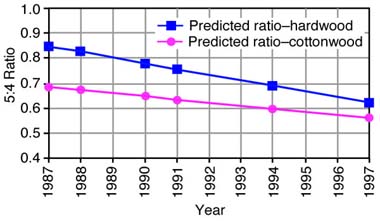
Fig. 23--Residual values for TM band 5:4 ratios for upland (hardwood) and bottomland (cottonwood) study forests at Fort Leavenworth, Kansas. Except for 1988, residual values for both forests fluctuate in similar ways.
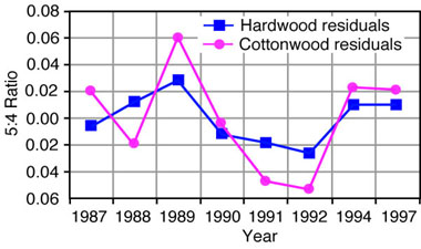
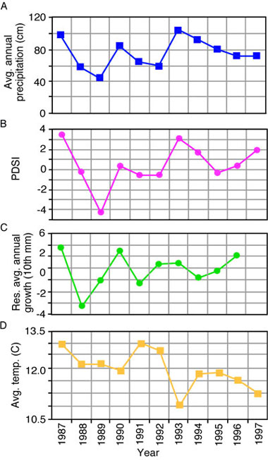
Table 6 presents data for climatic factors and average residual tree-ring widths for the study period 1987-1997. In 1988 and 1989, precipitation was far below normal, and the Palmer Drought Severity Index (PDSI) reached its lowest value in 1989. In 1991 and 1992, precipitation and PDSI values were also low. Tree-ring widths had the lowest (most negative) residual values in 1988, 1989, and 1991, during the two drought periods. In contrast, during 1987 and 1993, precipitation was over 100 cm (39 in) and PDSI values were greater than 3. The highest value for residual tree-ring width was in 1987, with high values also in 1990 and 1996. As fig. 24 illustrates, average precipitation, PDSI, and tree-ring residual width were generally in agreement; however, average temperature followed a different trend, generally opposite to precipitation and PDSI.
Table 6--Climatic and tree-ring data for Fort Leavenworth, Kansas, 1987-1997. Based on data from the National Climatic Data Center (NCDC, 1999) and Nang (1998). Mean annual 12-month periods are from July of the preceding year to June of the reported year; average residual tree-ring widths given in tenths of mm.
| Year | Mean Annual Precipitation (cm) |
Mean Annual Temperature |
Mean Annual PDSI |
Annual Residual Tree-ring Width (0.1 mm) |
|---|---|---|---|---|
| 1987 | 100.8 | 13.0 | 3.46 | 3.64 |
| 1988 | 58.0 | 12.2 | -0.28 | -6.42 |
| 1989 | 43.2 | 12.2 | -4.27 | -2.22 |
| 1990 | 84.8 | 11.9 | 0.34 | 2.94 |
| 1991 | 64.7 | 13.0 | -0.56 | -2.59 |
| 1992 | 59.0 | 12.7 | -0.58 | 0.67 |
| 1993 | 104.2 | 10.5 | 3.14 | 0.85 |
| 1994 | 93.1 | 11.8 | 1.69 | -1.63 |
| 1995 | 81.8 | 11.8 | -0.30 | -0.41 |
| 1996 | 72.9 | 11.5 | 0.39 | 2.11 |
| 1997 | 72.9 | 11.0 | 1.91 |
Fig. 24--Average annual precipitation (A), PDSI (B), residual tree-ring width (C), and average temperature (D) for the study period 1987 to 1997, Fort Leavenworth, Kansas.
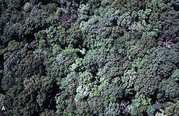
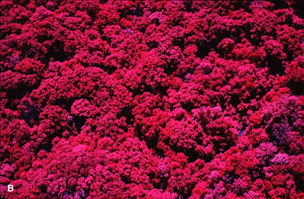
Photographs, both single-frame and stereo-pair modes, were taken with KAP repeatedly in normal color over the upland forest. Color-infrared images were taken in April and May 2000 and in June 2001. These various views reveal that the forest canopy is quite rough at a resolution of 1-10 m (3-33 ft) (fig. 25). Taller trees, mainly white oaks, extend several meters above neighboring trees, which creates numerous shadows in the canopy, when viewed from above. Vertical and oblique views reveal the upland forest has a closed canopy, except where openings exist for roads, trails, water tanks, or other human structures.
Fig. 25--Normal-color (A) and color-infrared (B) near-vertical views of the upland study forest, May 2000. Notice the rough canopy surface in which many shadows are present. The canopy completely covers the forest floor.
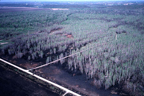
In April 2000, KAP was used to obtain images of the bottomland forest a few days after the adjacent grassland was subjected to a controlled burn. The same site was rephotographed one month later in May, and again in June 2001. The fire penetrated some distance into the forest understory, as shown on the April image (fig. 26). This burn took place at a time when the cottonwood trees had green flowers, but had not yet leafed out. The May images reveal that trees along the forest margin were injured by the fire. Some trees were completely bare, and others had leaves only in the upper portions or on one side. Trees within the main body of forest, however, were not affected by the fire.
Fig. 26--Normal-color, oblique view over the bottomland study forest, April 2000. The adjacent grassland was burned intentionally a few days before this picture, and the fire penetrated the forest understory some distance. At the time of this image, cottonwood trees had green flowers, but had not yet leafed out.
Prev Page--Methodology || Next Page--Interpretation and Discussion
Kansas Geological Survey
Web version January 25, 2002
http://www.kgs.ku.edu/Current/2002/aber/aber4.html
email:webadmin@kgs.ku.edu