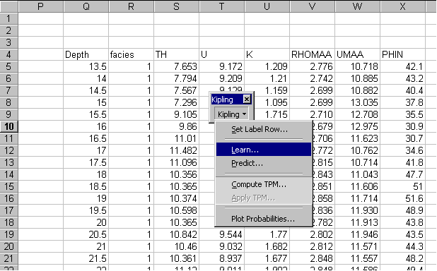

The prediction of a categorical variable will be illustrated using logs from the Lower Cretaceous in the Jones #1 well in north central Kansas. Core-based facies designations will be used to calibrate a model for predicting facies from six logs, including the thorium (TH), uranium (U), and potassium (K) values from a spectral gamma ray log, apparent grain density (RHOMAA), apparent matrix photoelectric absorption factor (UMAA), and neutron porosity (PHIN). The logs together with the core facies assignments can be seen here. Kipling requires that categorical values be specified as integers ranging from 1 to the number of categories. In this case the six facies are encoded 1 (Marine), 2 (Paralic), 3 (Floodplain), 4 (Channel), 5 (Splay), and 6 (Paleosol).
To start the training process we select the worksheet containing the facies designations and the log data and then select Learn... from the Kipling menu:

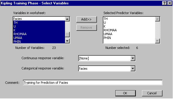
Then we choose the six logs as predictor variables and specify facies as our categorical response variable:
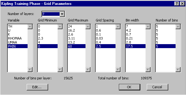
We now need to specify the discretization of the predictor variable space, as described in the theoretical background section and in the continuous variable prediction example. Here we specify a grid with around 25 grid cells along each axis and 7 layers of averaging bins:
The resulting histogram worksheet will contain bin-wise data counts for each of the six facies categories. These data counts provide an estimate of the relative prevalence of each facies in any particular region of the variable space defined by the six logs. Using this information, Kipling can compute a set of facies membership probabilities associated with a vector of measured log values. The worksheet created by the categorical prediction code contains columns of the membership probabilities associated with each log measurement in the prediction data set along with columns of facies (or category) indicator values, containing a "1" for the highest-probability category and a "0" for all other categories. Plots of the membership probabilities or facies indicators versus depth can be generated by first selecting Plot Probabilities... from the Kipling menu . . .
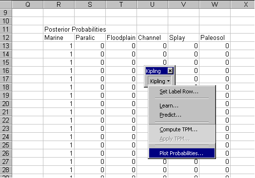
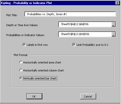
and then selecting the values to plot and the plot format . . .
The three plots below represent the original (core-based) facies assingments for the Jones #1 well, the probablities of facies membership based on re-substituting the log values into the model developed from the training process above, and the corresponding facies predictions:
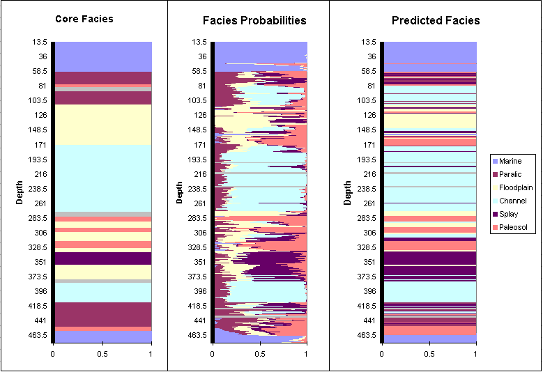
Although there is good overall agreement between observed and predicted facies in this case, the predicted sequence is quite erratic, with many short segments of facies interrupting the general sequence. This shortcoming can be remedied by incorporating transition probability information into the predicted probabilities of group membership.
Previous Page--Continuous Example ||
Kipling Home || Next
Page--Transition Probabilities