Kansas Geological Survey, Spatial Analysis Series 4, originally published in 1979

Originally published in 1979 as Kansas Geological Survey Spatial Analysis Series 4. This is, in general, the original text as published.
In recent years, statistical and mathematical techniques have been increasingly adopted within the geosciences. Geologists have originated few, if any, of the techniques; instead they have borrowed, adapted and used (or misused) them. In earlier papers (Tipper, 1977; Tipper, 1978) I attempted to introduce geologists to a number of additional techniques, chiefly from the field of Computer-Aided Design (CAD), which promise to be valuable in one of geology's most widespread problem areas—the study of complex three-dimensional shapes. This paper provides more comprehensive description and evaluation of these techniques, and attempts to develop a coherent framework to unite them with other techniques of shape analysis with which geologists are already familiar, e.g. trend surface analysis.
Studying the shape of three-dimensional objects and surfaces forms a major part of much geological work, and applications of shape analysis can be found in most branches of geology. Examples include delineation of subsurface mineral deposits, mapping of stratigraphical and structural surfaces, and investigation of the morphology of fossils. Because shape is so general a theme, it is essential that any methods developed for its study should be as efficient as possible. Furthermore, they should be independent of both the origin and geological meaning of the objects concerned.
We may classify methods of shape analysis into two major groups: methods of formal numerical analysis, and methods of mathematical (or statistical) surface representation. In the numerical methods, shapes are considered as points in a multi-dimensional space, the coordinate axes of which represent either variables or combinations of variables measured on the shape. In contrast, surface representation methods define an object by specifying its bounding surfaces, either by surface equations or, less commonly, by using statistical estimation techniques. These surface representation methods do no more than produce mathematical (and necessarily computerized) models of the objects: in consequence I refer to this approach by the general name "Computerized Modelling."
Most shape studies within geology have used the numerical approach. Methods used have included multivariate analysis (Gould, 1967, 1969; Blackith and Reyment, 1971; Brower, 1973; Demirmen, 1973), Fourier analysis (Ehrlich and Weinberg, 1970; Kaesler and Waters, 1972; Christopher and Waters, 1974; Delmet and Anstey, 1974; Gevirtz, 1976; Waters, 1977), and ad hoc descriptive methods such as have been developed for terrain analysis (Greysukh, 1966; Speight, 1968; Demirmen, 1973; Prelat, 1974). The great attraction of numerical methods is their operational simplicity, and this advantage is only lost on complex objects. (Here we consider an object to be complex if it has no obvious regularity of shape. Although a simple process may create a complex shape, we are interested more in the final shape than in the process by which it arose.) In practice the surface representation approach is the more efficient for objects with relatively complex curved surfaces, because it is much easier to specify surface equations than to define complex objects by such secondary measures as diameters or point-to-point distances. As the objects with which we shall be concerned in this paper are quite complex in form, only the surface representation approach is considered further here.
In describing the surface representation techniques, we shall attempt to indicate ways in which they can be compared one with another, both in theory and practice. The theoretical comparisons will be facilitated by maintaining consistent notation (Appendix 1), the practical comparisons by introducing an actual geological data set to which many of the methods will be applied. Before proceeding further we introduce this data set; in the rest of this study it is referred to as the Cherokee data set.
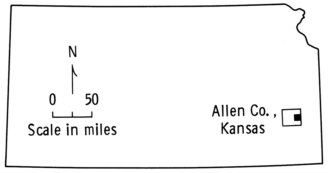
In southeastern Kansas, oil is produced from sandstones of the middle Pennsylvanian Cherokee Group. The reservoir sands form a complex subsurface meshwork; individual sands are impersistent laterally, "migrate" vertically, and frequently merge with one another. The sands in some areas are thought to have been laid down as channel deposits (McQuillan, 1968; Van Dyke, 1975), in other areas as offshore bars (Bass, 1936). Because of the history of its development, the oilfield studied (Fig. 1) provides an unusual volume of high-quality subsurface data. Each well has an associated gamma-ray log and, in most cases, has been cored through the producing interval.Figure 1—Location map showing area from which the Cherokee data set was obtained. Study area in Allen County, Kansas, is shaded.
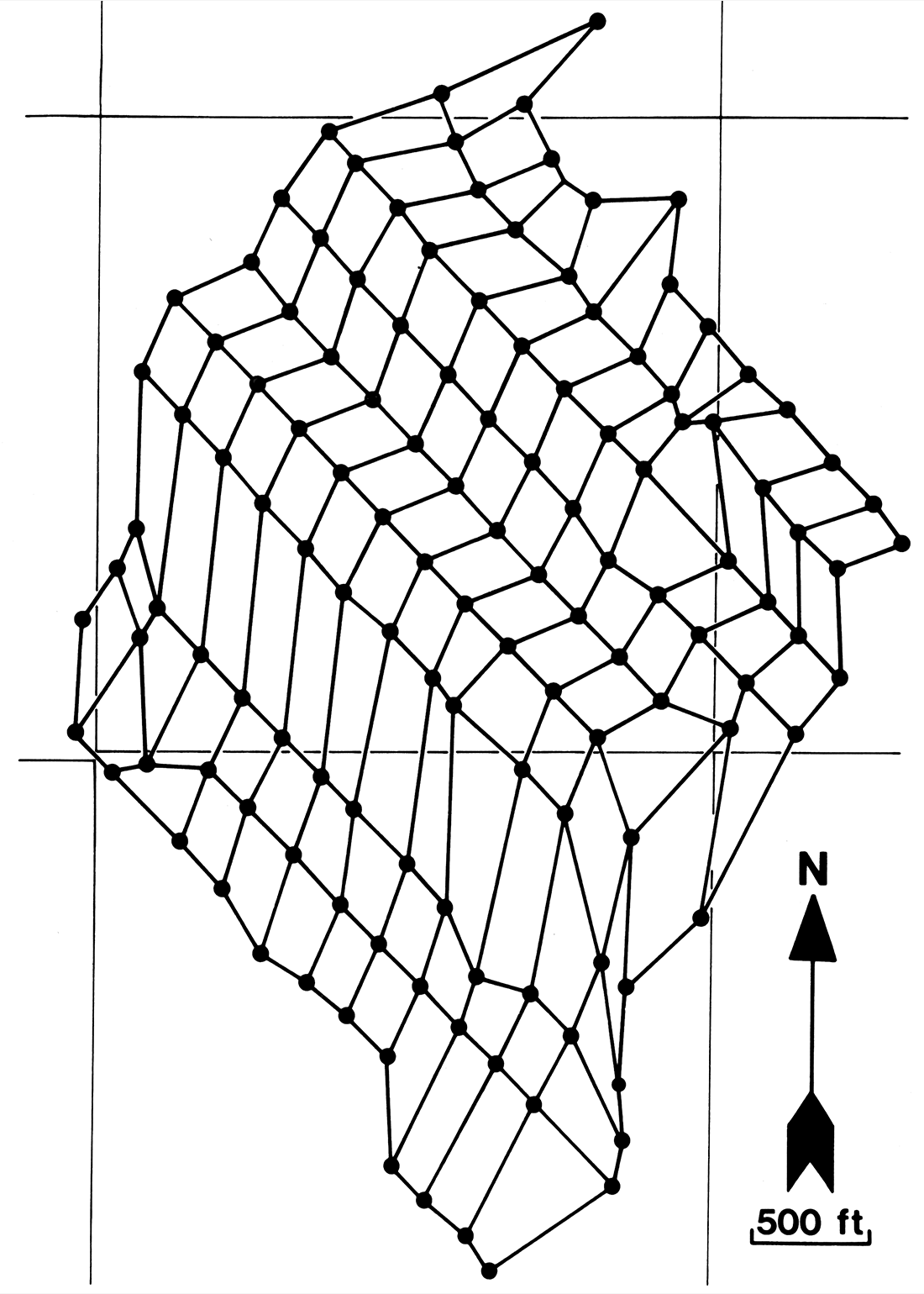
The actual data were obtained in the following manner. A set of 130 wells was selected, spaced on average at 100-metre intervals, and arranged on a (13-by-10) mesh (Fig. 2). The only restriction placed on the shape of the mesh cells was that they should be convex in plan view (cf. Hessing, et al., 1972). The top and base of each of four sands were picked from the gamma-ray log of each well, verified against the core descriptions where available, and a tentative correlation made for the entire well network. Where individual sand bodies could not be distinguished, as for instance when two superimposed sands had coalesced, arbitrary dividing horizons were chosen. In practice this introduces no problems provided that consistency is maintained. For simplicity in this present work only the two surfaces bounding one sand were retained. Thus the raw data consist of two sets of 130 height values (z) above sea-level datum, each value associated with position coordinates (x, y). These are given in Appendix 2.
Figure 2—Mesh of wells superimposed on 1/2-mile section grid. Each of the 108 cells in the (13-by-10) mesh is convex in plan view.
The reason for selecting this data set to illustrate a paper on shape analysis is that the three-dimensional form of the sands is of importance as a guide to additional drilling for tertiary recovery purposes. In the study area chosen, the subsurface is sufficiently complex that each sand unit must be studied independently. The problem is thus to develop ways to represent mathematically the bounding surfaces of each individual sand, and then to use these representations as bases for subsequent geological work.
Of the two steps involved here, the first is one of modelling, the second one of manipulating the models. In the remaining parts of this paper each step is considered in turn. Neither the treatment of the modelling process nor that of the manipulations which follow it pretends to be exhaustive. The methods described are a broad cross-section of those currently in use. References are given to the original sources (where known), and to important subsequent developments. So fast, however, is the field developing that any paper of this type must inevitably be incomplete. Realizing this, I have tried for balance at the expense of completeness.
Kansas Geological Survey
Placed on web Jan. 28, 2019; originally published 1979.
Comments to webadmin@kgs.ku.edu
The URL for this page is http://www.kgs.ku.edu/Publications/Bulletins/SpA4/index.html