| Original published in D. W. Steeples, ed., 1989, Geophysics in Kansas: Kansas Geological Survey, Bulletin 226, pp. 1-8 | ||
1Meridian Oil and 2TXO Production Corp.
The article is also available as an Acrobat PDF file.
A massive amount of information is available to the explorationist in the form of correlation-point seismic data recorded over the past 40 years, yet the archaic nature of the data inhibits its use. To the geophysicist trained in the modem technology of digital recording, computer processing, modeling, and seismic stratigraphy, these analog records are readily dismissed as being hopelessly outdated and incapable of containing any reliable information. To the geologist, they are just so many wiggles. An analysis of exploration targets and economics, however, reveals that these single-point records are the most cost-effective means of acquiring seismic information about the subsurface and when used within their limitations, correlation-point records can improve drilling success rates. Because of this, thousands of records are still being shot and recorded every year. In fact, this method of seismic exploration is the dominant method used today in Kansas. It is important then for the geologist and geophysicist to be able to recognize the utility and limitations of the tool and its role in prospect evaluation. This paper is intended to give the explorationist an exposure to the field-recording techniques, the data-reduction methods, and the mapping of shot-hole seismic records.
Seismic activity in the petroleum industry had its start in the late 1920's, shortly after it took hold in Texas and Oklahoma. Extensive mapping was done on the Cimarron anhydrite by the spring of 1929 (Weatherby, 1948), by which time several seismic crews were actively recording reflection data. By the time seismic exploration had come into common use in the 1930's, Kansas' six major oil fields had already been discovered (Pratt, 1959). As the Kansas petroleum industry developed, seismic-exploration methods improved and came to play an increasingly important role in the discovery of new reserves. A review of the Kansas Geological Society Oil and Gas Fields volumes 2 and 4 shows that 38 of the 64 fields listed in western Kansas credited seismic data as their source of discovery.
It would be a formidable, if not impossible, task to compile figures on all of the wells drilled from shot-hole seismic data recorded over the past 50 years. Hundreds of thousands of seismic records have been preserved and are available today from data brokers. Thousands of shotpoints are still being recorded every year. Those who understand the applications and limitations have a valuable tool to use in their search for oil.
In order to understand the use of single-point or shot-hole data, awareness of the field methods used in acquiring the data and how to convert the field data to usable information is necessary. This in turn results in an appreciation of how the shot-hole records are used for mapping the subsurface.
The basic field setup for recording seismic reflections is to array a series of geophones at the earth's surface to record the sound energy from an explosive source. A number of geophones are used to record each of a number of seismic traces. The multiplicity of geophones tends to reduce the unwanted portion of the reflection train, or noise, improving the overall signal-to-noise ratio.
Correlation-point seismic data are recorded with the geophones arrayed close to the shot hole (fig. 1A). With this setup, each shotpoint is independent of the others with no traces in common with any of the shotpoint records in a survey area. This independence allows the data to be displayed with some variety. The same traces may be shown on a record several times, each with a different filter, allowing the interpreter to evaluate the consistency of reflectors. The typical seismic record is designed to display 24 traces. The same eight traces may be displayed with three filters, or the same 12 traces may be displayed with two filters. Most correlation-point data are shot in an off-end array with the geophones extending away from the shot hole in one direction. This allows for the eight-trace, three-filter display.
Figure 1--Shotpoint arrays and subsurface coverage: A) Off-end spread, B) Split spread, C) Continuous profile. Subsurface coverage is one-half the surface-measurement distance by the principle of equal-angle incidence and reflection raypaths. When surface coverage overlaps by 50% or greater, subsurface coverage is continuous.
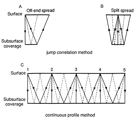
The other frequently used setup for correlation-point recording is the split-spread where geophones are placed in two sides of the shot hole (fig. 1B). Typically, six traces are arrayed on each side of the hole with the resulting 12 traces displayed with two filters. One advantage to this method is the additional information of two near-traces. Seismic times may be averaged across the shot hole for more reliable values.
The 100% method of seismic recording is an extension of the split-spread, correlation-point setup (fig. 1C). The shot hole and geophone locations are positioned so that the far traces of adjacent shotpoints record data reflected from common subsurface positions. This allows for the direct correlation of reflections from shotpoint to shotpoint and is especially helpful where more complicated structures such as faults are anticipated. The extension of the 100% setup is the common depth point, or CDP, recording where more than one trace per shotpoint is common with adjacent shotpoints. The 100% method requires the additional survey information of elevation and position for the individual geophone groups. The far traces of each shotpoint require datum corrections similar to the near-traces in order to correlate from shotpoint to shotpoint. The additional information from a 100% survey is useful in calculating weathering-thickness changes.
Fig. 2 is a typical shotpoint header and upper portion of a shot-hole record. On this portion of each correlation-point and 100% seismic record are all of the field data necessary to correct the shotpoint to a reference datum. Each shotpoint is adjusted to the datum so that zero time is equivalent to all other zero times in the survey. This in turn enables a correlation between shotpoints and geologic formations in well bores.
Figure 2--Typical off-end correlation-point seismic record: A) Time break, B) Uphole time, C) Shotpoint elevation, D) Charge depth and size, E) Shotpoint location, F) Filters, G) Zero time line, H) Datum correction, I) Spread configuration, J) Velocities used to compute Tc, and K) Drill log.
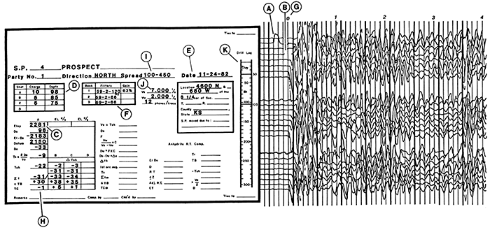
The time break, TB or Tb, is the response generated by the charge detonation (fig. 2A). The direction of the time-break deflection is usually opposite the direction of the first energy arrivals. The uphole time, Tuh, is the travel time for the charge energy to reach a geophone at the earth's surface at the shotpoint location (fig. 2B). The elevation of the shotpoint is given as well as the charge depth and size, the shotpoint location, and filters used (fig. 3C-F). Most of these data are used in calculating datum corrections and depths of weathering. The zero-timing line (fig. 2G) may be selected arbitrarily on the record or cued to the time break. All times on the record are measured from this zero timing line. The basic datum correction is calculated using the "normal" uphole calculation, its name referring to both the ease of the calculation and the assumption that seismic energy travels at normal incidence through the subsurface formations and is not refracted at the formation boundaries.
The "normal" uphole calculation is
Tc = Te - Tuh + Tb
where
Tc = time correction
Tuh = uphole time
Tb = time break
and
Te = 2De/Ve
where
De = (Elsp -Ds) - Eld
and Eld = datum elevation
Elsp = shotpoint elevation
Ds = shot depth
Figure 3--Explanation of parameters used in datum corrections: Elsp = Shotpoint elevation, Tuh = Uphole time, Ds = Shot-hole depth, Vw = Weathered-zone velocity, Ve = Estimated velocity of consolidated sediments, De = Elevation difference between shothole depth and datum plane, Dw = Depth of weathering.
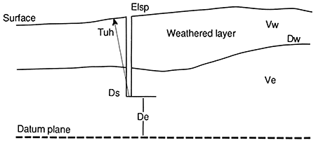
Determining a surface correction as shown in fig. 3 can be done with a simple geometric approach. The modified uphole calculation expands upon the normal uphole method by incorporating a correction for the refraction of the seismic energy at the weathering-subweathering interface. To avoid the tedium of calculating through Snell's law every time a correction is to be made, tables of factors are available to facilitate the computation.
Other styles of computing datum corrections are available based on experience in data reduction and personal preference.
Depth of weathering, Dw, can be calculated using the relationship of
Tuh = Dw/Vw + (Ds-Dw)/Ve
to determine that
Dw = (Tuh-VwDs / VeVw) (VeVw / (Ve - Vw))
This calculation is useful in designating secondary charge depths for successive records at the same shotpoint. The depth of weathering is also useful in itself for other studies, especially refraction-statics calculations as well as general data-quality problem recognition.
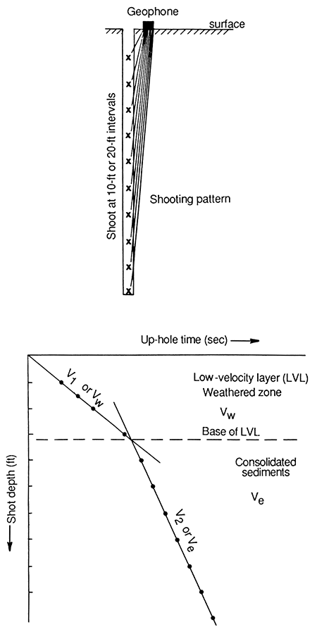
Throughout the above calculations, Ve and Vw are used. These values are average velocities and were initially determined by recording uphole-velocity surveys (fig. 4). These surveys consist of detonating dynamite charges at regular intervals in a deep shothole, with a geophone located at the surface. The charges are detonated with the geophone recording the numerous uphole times. The times and charge locations are plotted to determine the velocities of the weathered and consolidated zones. These velocities are found to vary over the state, but the effect of the variation is insignificant for all but the largest surveys. A list of wells shot for velocity is published annually by the Society of Exploration Geophysicists.
Figure 4--Schematic view of uphole velocity survey with corresponding plot of data to determine Vw and Ve. Survey may be performed with shots in the hole and geophones on the surface or with geophones in the hole and energy source at the surface.
Reflection times are taken directly from the shothole record relative to zero time. They are usually read from the nearest traces of the shotpoint because the datum-correction calculations are most applicable at the shotpoint location and not to the traces at a distance from it. No compensation is made by normal moveout on the outer traces rendering them most useful for correlating reflections through noise. However, the far traces of 100% data are corrected to the datum allowing for correlation from shotpoint to shotpoint in the presence of normal moveout. Phase lags, inherent in the frequency-dependent filters of analog equipment, affect the reflection times seen in each filter bank of the record. This requires consistency in the selection of the filters used for interpretation from shotpoint to shotpoint and from survey to survey.
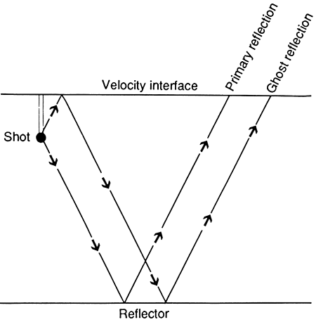
When multiple shots are taken in a shot hole, differences occur in reflection character, primarily a result of the competency of the material in which the charge is placed. The depth-of-charge placement greatly influences the strength of the interference of multiple reflections, or source ghosts (fig. 5). The source-ghost reflection is often responsible for more variation in record character than any other factor (Hammond and Hawkins, 1958). Because it lags the primary reflection, the source ghost appears as an event just below a primary reflector and with reduced amplitude. A comparison of equivalent reflections on records from different shot depths for a given shotpoint often reveals the occurrence of ghost reflections. It is important to recognize ghost reflections to avoid mapping them.
Figure 5--Propagation of ghost reflections from earth-air interface.
Care must be taken when correlating reflections on seismic records of different vintage or operator, or on records which may have been reproduced a number of times through a data-brokerage service. Timing line spacing may not be the same from record to record, resulting in miscorrelation.
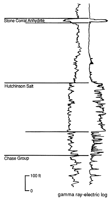
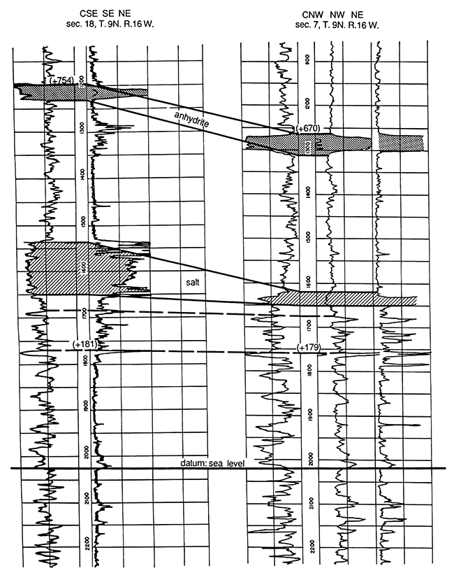
In western Kansas, correlation of shot -hole records is aided greatly by the occurrence of a strong reflection from the Stone Corral Formation. This Lower Permian unit is composed primarily of anhydrite, with dolomite and shale members. It blankets western Kansas (Merriam, 1963) at sufficient depth to generate a reflection below the near-surface noise zone. The Stone Corral is a high-velocity material encased in a lower velocity shale section, giving it a large reflection coefficient. The average velocity to the anhydrite is approximately 8,000 ft/sec (2,400 m/sec) along the western flank of the Central Kansas uplift, increasing to approximately 9,000 ft/sec (2,700 m/sec) near the Colorado border. Identification and correlation of deeper reflections are facilitated by the alignment of the anhydrite reflections. Where the Stone Corral is absent or too near the surface to detect seismically, other horizons are used for mapping purposes. Several limestones in the Wabaunsee Group are identifiable by their strong reflections, and their occurrence below the Permian strata render them useful in detecting prePermian structures. The Hutchinson Salt Member of the Permian-age Wellington Formation lies below the Stone Corral (fig. 6) and exhibits not only lithologic changes but also flowage (Kulstad, 1959), causing the Stone Corral to collapse or slump over the salt-thickness changes. This can cause a change in interval time between the Stone Corral and deeper horizons which is not related to deeper structures. Mapping deeper intervals can uncover problems associated with salt instability.
Figure 6--Typical electric-log response from Permian formations affecting shallow velocities.
The standard approach to mapping shot-hole data involves the use of interval-travel times to construct maps of isotimes similar to isopach maps of the subsurface. This is necessary because the inherent uncertainty in weatheringtime corrections may be greater than the time relief of the geologic structures being sought. Most of Kansas is covered by a weathering layer that displays inconsistent thickness and velocity. Structural datum corrections may not correct for all of the local weathering changes, resulting in mistaken ties with known formation depths. The interval times between reflections are not as severely affected by changes in the nearsurface, allowing for closer correlation with well tops and a higher degree of reliability where there are no other subsurface data.
Interval-time decrease or thinning is generally associated with deeper structural highs. This arises from the basic assumptions that thinning occurs in the sedimentary layers draping deep-seated structural highs and that the thinning is preserved through unconformable sequences of deposition. In local survey areas, the Stone Corral is assumed to have been deposited as a flat-lying unit. Thinning between the Stone Corral and deeper reflectors, then, can depict structures which existed when the anhydrite was deposited. In a similar manner, thinning between successively deeper reflections can indicate structural episodes in the depositional sequence of the survey area.
Time-structure maps are usually constructed for the upper reflector used in isotime mapping. These maps are critical in helping determine that mapped thinning is due to deep structure rather than to a structural low in the upper surface. The reliability of the time-structure map is determined by how accurately it depicts the structural attitude of the reflecting horizon compared with the geologic information available, most commonly well logs.
A number of geologic horizons are mappable over a large area with shot-hole seismic data. An approximation of the potential to reflect seismic energy for particular formations is shown in the synthetic seismogram in fig. 7, constructed from a sonic log with known formation depths. In addition to the Stone Corral and other Permian-age formations, the Wabaunsee, Lansing, and Mississippian limestones may be detectable by their consistent reflections. The synthetic seismogram offers the most accurate means of identifying reflectors. Where velocity logs are unavailable, reflectors may be identified somewhat less accurately using average velocities from the available control.
Figure 7--Identfication of reflectors is greatly enhanced by the use of synthetic seismograms such as this, which are constructed from sonic logs to simulate seismic responses of the subsurface.
In areas of suspected near-surface velocity anomalies, or where the anhydrites and other younger beds are shallow or absent, an additional tool is available to the seismic interpreter. Electrical logging of the shot holes in a survey can give valuable information about the dip and occurrence of near-surface beds. Shot-hole driller's logs frequently indicate the depths at which different shallow formations are encountered. Mapping these data can give insight into the structural attitude of formations used for interval mapping. The most important subsurface information to be used in a seismic survey is from wells drilled in the area necessitating well ties with the shot-hole survey, whether new data or vintage records. A number of well ties in a survey area provide a check of the reliability of the shotpoints. They also provide the depths to the target formations, helping to determine which maps are most useful to evaluate the prospect.
Many modern computer-processing techniques are applicable to data shot in continuous 100% format. Paper records and FM field tapes may be transcribed to digital format on magnetic tape by manual or optical digitizers. This makes available all of the current data-processing methods used in CDP seismic processing. Normal moveout, statics, and velocity corrections are determined, and the data are filtered for display in section format similar to CDP profiles. Waveform character may be enhanced with deconvolution filters. Section format display allows for flattening and coherency filters to be applied (Lambright, personal communication, 1984).
Shot-hole data can complement CDP shooting in a variety of ways. The near-surface weathering information is useful in refraction-statics processing. Mapping the data can reveal the regional dip of the survey area for planning line placement. Shot-hole data also offer an inexpensive method to determine the seismic response of the formations in the survey area. Even the identification of poor data areas is useful when determining the recording parameters, despite the frustration of having to work with the deteriorated record quality.
As the size of the exploration targets in Kansas decreases, the single-point method continues to gain importance as an exploration tool. It offers a cost-effective means of acquiring subsurface information of sufficient density to delineate drillable prospects. It can accurately map formations which are the most influential ones in hydrocarbon accumulation and entrapment. Modern CDP seismic methods offer advantages in the exploration for stratigraphic targets. But the inherent redundancy of the method and, consequently, its high price tag limit its applications. The advantages of the economy and greater areal extent of the single-point format are offset by the lack of noise reduction and character development. Yet shot-hole seismic processing is easily the dominant method being used in Kansas today. The abundance of available vintage data allows the exploration dollar to be spread over several prospects at a fraction of the current acquisition costs. These features ensure that the single-point method will maintain its prominence in the Kansas petroleum industry, its usefulness to be determined by those who understand its applications and limitations.
The authors wish to thank the following persons for their patience and for sharing the benefits of their experience: Bill Hamm and Lucky Opfer of Exploration, Inc.; Herman Schmalz of Classic Exploration; Howard Schwertfeger of Geosearch, Inc.; Warren Heatley of Reliance Exploration; Carter Davis and Orbie Lambright of Geoscan Services Company.
Hammond, J. W., and Hawkins, J. E., 1958, Getting the most out of present seismic instruments: Geophysics, v. 23, no. 4.
Kulstad, R. O., 1959, Thickness and salt percentage of the Hutchinson Salt; in, Symposium on Geophysics in Kansas: Kansas Geological Survey, Bulletin 137, p. 241-248. [Available online]
Merriam, D. F., 1963, The geologic history of Kansas: Kansas Geological Survey, Bulletin 162, 317 p. [available online]
Pratt, W. E., 1959, Foreword; in, Symposium on geophysics in Kansas: Kansas Geological Survey, Bulletin 137, p. 6-8. [Available online]
Weatherby, B. B., 1948, Early seismic discoveries in Oklahoma: Geophysical Case Histories, v. 1.
Kansas Geological Survey
Comments to webadmin@kgs.ku.edu
Web version July 20, 2013. Original publication date 1989.
URL=http://www.kgs.ku.edu/Publications/Bulletins/226/McGuire/index.html