Principal Component Analysis Brine Data

"Principal component analysis (PCA) is a statistical procedure that uses an orthogonal transformation to convert a set of observations of possibly correlated variables into a set of values of linearly uncorrelated variables called principal components. The number of principal components is less than or equal to the number of original variables. This transformation is defined in such a way that the first principal component has the largest possible variance (that is, accounts for as much of the variability in the data as possible), and each succeeding component in turn has the highest variance possible under the constraint that it is orthogonal to the preceding components. The resulting vectors are an uncorrelated orthogonal basis set. The principal components are orthogonal because they are the eigenvectors of the covariance matrix, which is symmetric. PCA is sensitive to the relative scaling of the original variables."
Wikipedia, the free encyclopedia (https://en.wikipedia.org/wiki/Principal_component_analysis)

Brine Data - Principal Components Analysis

The original Brine data set are converted from mg/l units to meq/l units.

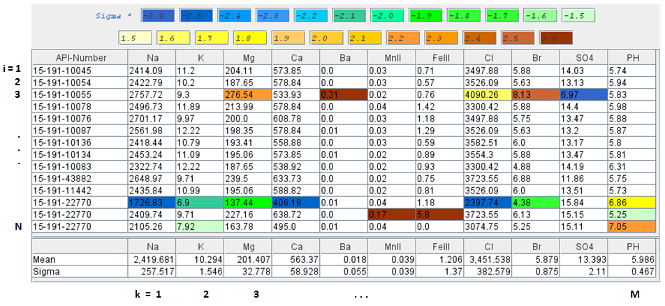
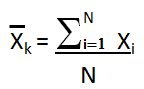
Mean X̄_k is the average value of each column k

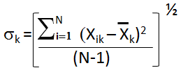
Sigma (Standard Deviation) σ_k is a measure of how spread out the kth data column is

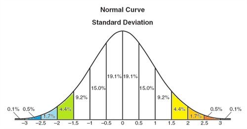
The brine data cells are colored to illustrate how spread out the data is with respect to the standard deviation, i.e. green and blues from -1.5σ to less than -3σ and yellows and oranges from 1.5σ to above 3σ. Normalize each column to its standard deviation. Unless the data is normalized, a variable with a large variance will dominate, x_ik = X_ik/σ_k , where i is the row, k is column.

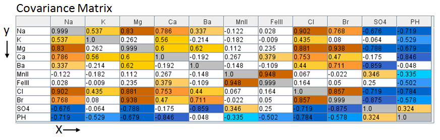
The web app performs all the processing in the background. The process begins by constructing the Covariance matrix for the brine data set. Covariance [cov(x,y)] matrix is a measure how much each data column vary from the mean with respect to each other.

where x is the mean of brine data column k divided by σ_k where x_i is the individual brine data divided by σ_k, subscript i represents the well, subscript k represents the brine data column, e.g. cov (Na, Ca) is sum over the Na (Sodium cation) and Ca (Calcium cation) columns of the normalized data set.

To compute the Eigenvectors and Eigenvalues this web app uses JAMA a Java Matrix Package (http://math.nist.gov/javanumerics/jama/ ).

"JAMA is a basic linear algebra package for Java. It provides user-level classes for constructing and manipulating real, dense matrices. It is meant to provide sufficient functionality for routine problems, packaged in a way that is natural and understandable to non-experts. It is intended to serve as the standard matrix class for Java."

JAMA Java Functions:
C represents the symbol for the Covariance Matrix
The eigenvalues & eigenvectors JAMA functions are listed as follows
   Ev = C.eig(), where the eig() function computes the eigenvalues & eigenvectors of the covariance matrix C.
   Eigenvalues  = Ev.getRealEigenvalues()
   Eigenvectors = Ev.getV().

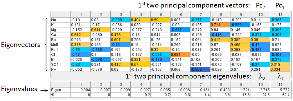
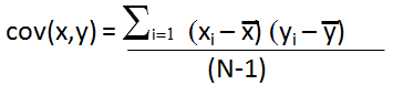
The principal components is less than or equal to the number of original variables. The first principal component Pc₁ has the largest possible variance i.e., it accounts for as much of the variability in the data as possible and the next principal component Pc₂ has the highest variance possible under the constraint that it is orthogonal to the preceding component. The principal components are orthogonal because they are the eigenvectors of the covariance matrix, which is symmetric.

Construct a Feature Vector from the 1st two principal components, e.g. columns 10 and ll.

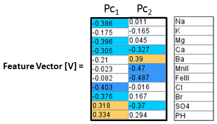
Then construct an Adjusted Data Matrix from the Brine Data Matrix by subtracting the mean of each column and then dividing the standard deviation of the each column.

Adjusted Data Matrix [Am] = [ (X_ik - X̄_k) / σ_k ]

where X̄_k is the mean of the brine data column k,
           X_ik is the individual brine data; i = well, k = brine data column,
           σ_k is the standard deviation of the brine data column.

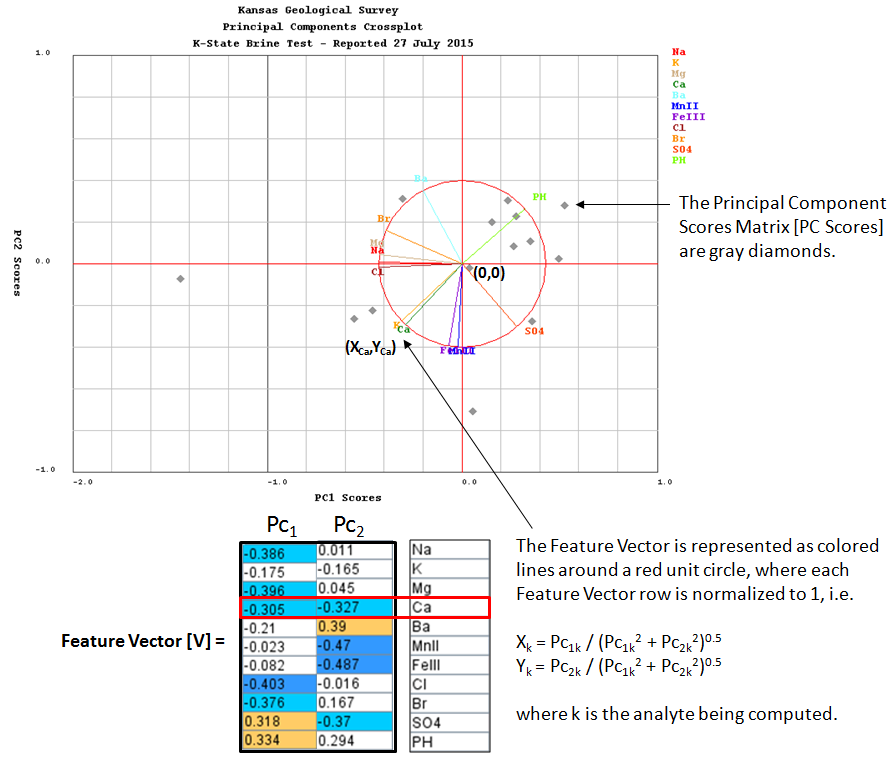
Compute the Principal Components Scores [PC Scores] matrix as the Adjusted Data matrix times the Feature Vector.

           [PC Scores] = [Am] X [V]

The Principal Components Scores [PC Scores] matrix converts the multi dimensional matrix into a 2 dimensional matrix.

References A tutorial on Principal Components Analysis by Linsay I Smith February 26, 2002

Author: John R. Victorine jvictor@kgs.ku.edu

The URL for this page is http://www.kgs.ku.edu/PRS/Ozark/Software/PC/index.html