Kansas Geological Survey, Open-file Report 2000-40
Part of the Well Tests for Site Characterization Project
by James J. Butler, Jr.
Kansas Geological Survey
1930 Constant Avenue, Campus West
Lawrence, KS 66047
and
Elizabeth J. Garnett
Department of Geology
University of Kansas
Lawrence, KS 66045
KGS Open File Report 2000-40
December 2000
The purpose of this report is to describe two simple approaches for analysis of slug tests in formations of high hydraulic conductivity. These methods are straightforward implementations of models described by Springer and Gelhar (1991) and Butler (1997) for slug tests performed in wells that partially penetrate unconfined and confined formations, respectively. These approaches have been devised to make the analysis procedure for slug tests in highly permeable formations more accessible to the field practitioner. Both approaches involve the graphical matching of theoretical type curves to plots of slug-test response data. The first approach is a spreadsheet-based procedure using the Excel software package (Microsoft, 1997), while the second utilizes any of a number of scientific-graphics packages. Given the speed with which the analyses can be performed, no attempt has been made to fully automate these procedures. The files needed to implement these approaches are included with this report, and both methods are illustrated using test data from a field site of the Kansas Geological Survey.
The two procedures described here for the analysis of slug tests in formations of high hydraulic conductivity implement straightforward extensions of models previously proposed for tests in less-permeable formations (Bouwer and Rice, 1976; Hvorslev, 1951). The model of Springer and Gelhar (1991) is used for the analysis of tests in unconfined aquifers, while the model designated in Butler (1997) as the linearized variant of the McElwee et al. (1992) model is used for tests in confined aquifers. For the remainder of this report, these models will be designated as the high-K Bouwer and Rice and high-K Hvorslev models, respectively, to emphasize their relationship to those earlier models and to the quasi-steady-state assumption upon which they are based (Butler, 1997).
Regardless of which procedure is used or whether the test has been performed in an unconfined or confined aquifer, the general approach for the processing and analysis of slug-test response data is the same. The approach consists of the following four steps:
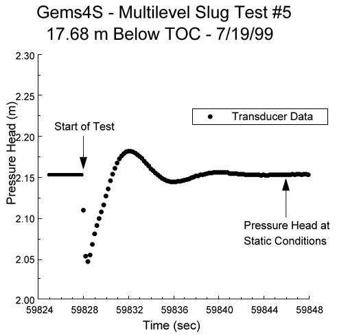
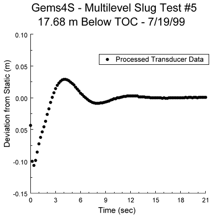
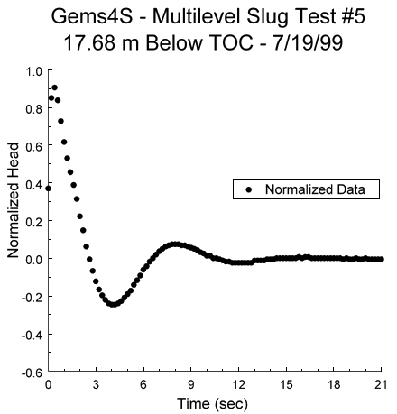
1) Pressure transducer readings are plotted versus the time since some arbitrary starting point (Figure 1A). The time at which the test began and the pressure head corresponding to static conditions are identified from this plot. The static pressure head and the test start time are then subtracted from the head and time records, respectively, to obtain a plot of the deviation of the pressure head from static conditions (designated in this report as H(t)) versus the time since test initiation (Figure 1B). As is the convention for slug tests, the deviation data are normalized using the change in water level (H0) that initiated the test (Figure 1C). For tests initiated with the pneumatic method (e.g., Butler, 1997), the initial displacement is best estimated from the air-pressure transducer readings;
Figure 1a. Example plot of the pressure head versus the time since some arbitrary starting point (in this case, 12:00:00 AM).
where
CD = dimensionless damping parameter;
g = gravitational acceleration;
H0 = change in water level initiating a slug test (initial displacement);
Le = effective length of water column in well;
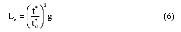
td = dimensionless time parameter,
![]() ;
;
t = time;
w = deviation of water level from static level in well;
wd = normalized water-level deviation (w/H0);
![]() = dimensionless frequency parameter
= dimensionless frequency parameter
![]()
![]()
Figure 2. Normalized deviation from static (w/H0) versus dimensionless time type curves (CD defined in text).
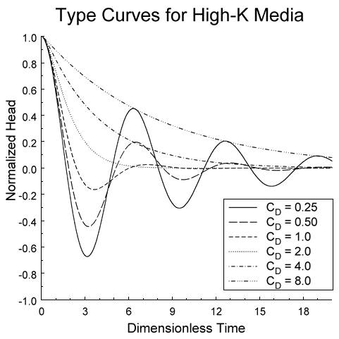
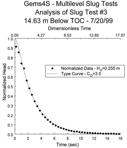
Figure 3a. Superposition of type curve and normalized data plots (type curve plots reference upper x-axis while normalized data plot references lower x-axis; every second data point plotted).
Unconfined--High-K Bouwer and Rice Model (Springer and Gelhar, 1991)
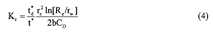
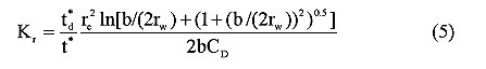
Although these equations are based on the assumption of an isotropic aquifer, an anisotropic form of either equation can be obtained through modification of rw as described by Zlotnik (1994). In that case, rw in equations (4)-(5) is replaced by rw* ( , where Kz is the vertical hydraulic conductivity). Note that the unconfined model, equation (4), applies for wells screened away from or up against an impermeable lower boundary. The position of the screen with respect to the boundary is considered in the calculation of the logarithmic term (Bouwer and Rice, 1976). However, the confined model, equation (5), does not apply for wells in which the screen abuts an impermeable boundary. In that case, a modified version of the Hvorslev model should be used in which the 2rw terms in the numerator of equation (5) are replaced by rw.
The definition of dimensionless time following equation (3) includes a parameter designated as the effective length of the water column (Le). Zurbuchen et al. (in press) and others have analyzed slug-test response data assuming that this quantity can be computed from well-construction parameters and assumed known for the analysis. That approach, however, generally does not produce a good match between the type curve and the response data, indicating that the relevant physical processes are not completely described with the definition of Le used by those previous workers. Given the complexity of slug-induced flow in a well screened in a highly permeable aquifer, it is difficult to account for all contributions to the Le term. Thus, in the procedures described here, Le is calculated as part of the analysis process (Butler, 1997):
The type curves of Figure 2 represent the theoretical deviation of the water level from the static position in the well. The general approach outlined in the preceding paragraphs is based on the assumption that a pressure transducer in the water column will provide an accurate record of the water-level position. However, Zurbuchen et al. (in press) have recently pointed out that a transducer may not provide an accurate record of water-level movement in conditions of high water column accelerations. The accuracy of the apparent water-level record obtained from a pressure transducer in an accelerating water column is a function of, among other things, the length of the water column above the transducer. The further the transducer is below the static level, the less accurate the record of water-level movement. Zurbuchen et al. (in press) proposed the following type-curve correction to account for the position of the transducer in an accelerating water column:
![]()
Hd(td)* = theoretical normalized head corrected for transducer position;
ptdepth = depth of pressure transducer below static
![]() = second derivative of wd with respect to time.
= second derivative of wd with respect to time.
The depth of the pressure transducer below static is measured in the field and the second derivative of the type curve is computed either analytically or using a simple finite-difference scheme. Since this correction requires an estimate of Le, which, as discussed in the previous paragraph, is usually not known, error can be introduced into the correction process. Fortunately, as shown by the form of Equation (7), the need for this correction can generally be avoided by placing the transducer very close to the static level (within 0.5 m).
Equations (4) and (5) have been presented as models for use in highly permeable formations. However, these models can also be used for tests in less permeable formations. In that case, equations (4) and (5) will be equivalent to the conventional forms of the Bouwer and Rice (1976) and Hvorslev (1951) models, respectively. Although the type-curve method presented here can be used for analysis of tests in less permeable formations, it is less efficient than the standard approach of fitting a straight line to a log normalized head versus time plot. Thus, this method should not be used when analysis methods developed for less permeable formations are a viable alternative. Kipp (1985) shows that analysis methods for slug tests in less permeable formations are valid for CD values greater than about 10.0. As Butler (1997, p. 150) points out, a linear or concave-upward character to a log normalized head versus time plot is an indication that the specialized methods developed for highly permeable formations are not needed.
This general approach for the processing and analysis of response data from slug tests in highly permeable aquifers is implemented in both procedures discussed in this report. These two procedures are described in detail in the following sections.
Procedure One--Excel Spreadsheets
This approach is implemented using two spreadsheets in the file High K Slug Tests.xls. Spreadsheet Type Curve Generator is used to generate type curves with equations (1)-(3), while spreadsheet High K Estimator is used to process and analyze the slug-test data. The workings of each of these spreadsheets will be briefly described in this section. Note that the processing and analysis of individual tests can be readily completed within five minutes using this procedure.
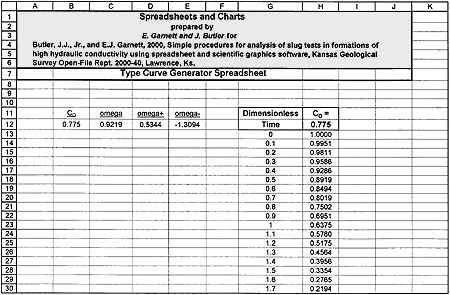
Figure 4A is a view of a portion of spreadsheet Type Curve Generator. The CD value for which a type curve is to be generated is entered in cell B12. The theoretical normalized responses are then calculated in column H using the appropriate equation (equations (1)-(3) depending on CD value). Values for the various frequency parameters appearing in equations (1)-(3) are also calculated and given in cells C12-E12. A plot of dimensionless time versus the theoretical normalized response (type curve) is automatically generated as Chart 1.
Figure 4a. View of a portion of spreadsheet Type Curve Generator. A larger version of this figure is available.
Procedure Two--Scientific Graphics Software
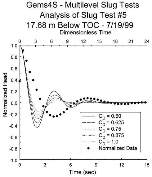
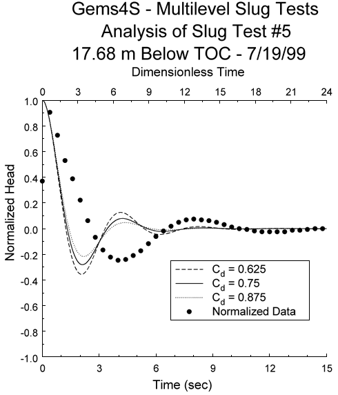
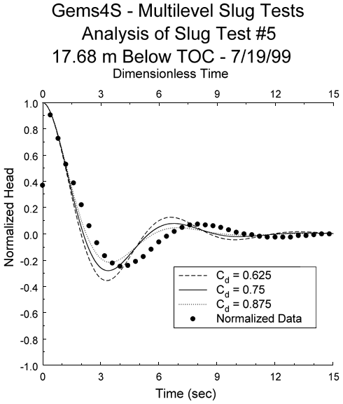
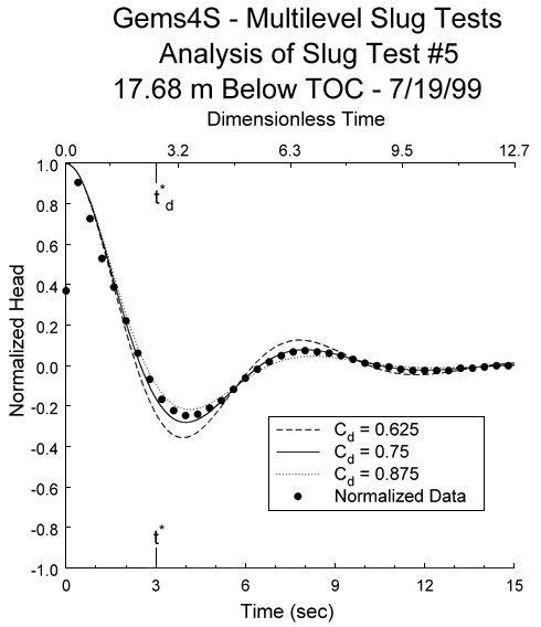
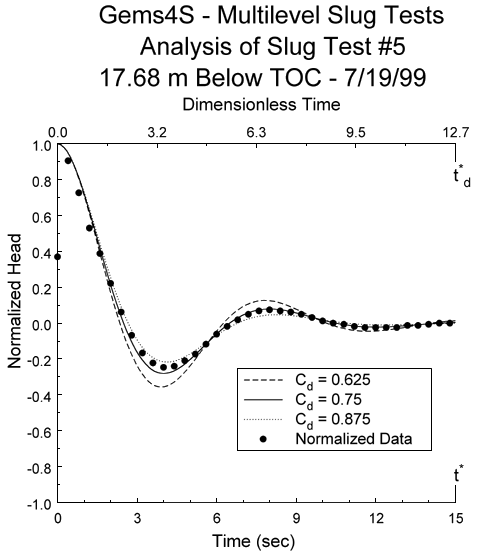
This approach can be implemented using any of a number of scientific-graphics packages. Axum 5.0 (MathSoft, 1996) was used here. The processing of the response data (Figures 1A-1C) can be readily done using the data-transformation option standard in scientific-graphics software. The analysis of the response data is performed using a library of type curves and the graphics capabilities of the software. The type curves are superimposed on the plot of the response data as shown in Figure 3A. The type-curve plot references the upper x-axis, while the response-data plot references the lower x-axis. The range of type curves relevant for the analysis is readily determined from this initial graph. All type curves outside of this range are hidden from view using a standard option available in scientific-graphics software (Figure 3B). The curve match is obtained by continually changing the maximum value of the x-axis referenced by the type-curve plot until the type-curve and data plots essentially coincide (Figures 3B-3D). The CD value and time match points (td* and t*) are then selected and substituted along with the well-construction parameters into the appropriate equation to obtain an estimate for Kr. As with the Excel-based approach, the processing and analysis of individual tests can be readily completed within five minutes using this procedure. Potentially, the most difficult aspect of the procedure is the determination of the match points on the time axes. Although any arbitrary points can be selected (e.g., Figure 3D), the simplest approach is to use the maximum values for the two x-axes since those can be read directly off the graph (e.g., Figure 3E).
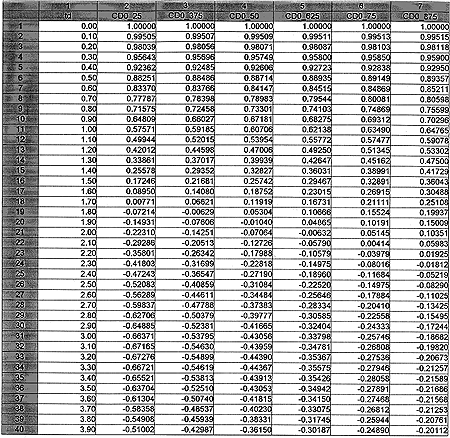
The type curves needed to implement this procedure are included with this report. If the response data are oscillatory in character, the file named hiK1.dat should be used. This file has type curves for CD values between 0.25 and 2.0 at 0.125 increments. If the response data are not oscillatory in character, the file named hiK2.dat should be used. This file has type curves for CD values between 2.0 and 10.0 at increments of 0.25 from 2.0 to 5.0, 0.50 from 5.0 to 8.0, and 1.0 from 8.0 to 10.0. An example of the format of the type-curve files is given in Figure 5. If response data fall between two of the type curves, a CD value can be estimated via interpolation (e.g., Figure 3D) or additional curves can be readily generated with the data-transformation capabilities of scientific-graphics software. Since interpolation will introduce little error into the procedure, it is the recommended option. Generation of additional type curves should only be considered in cases where the CD value is quite small (<0.5). Note that the type curves in hiK1.dat and hiK2.dat can be used for wells screened away from or up to an impermeable boundary.
Figure 5. Example format for type-curves files hiK1.dat and hiK2.dat. A larger version of this figure is available.
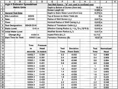
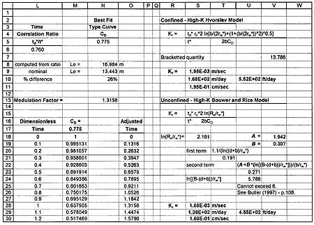
Oscillatory Response Data--Figure 6A displays the normalized head versus time plot for three of a series of slug tests performed in a confined coarse sand and gravel aquifer underlying the Kansas River floodplain near Lawrence, Kansas (Butler et al., in review). The coincidence of the normalized plots indicates that dynamic-skin effects and dependence on the magnitude of the initial displacement can be neglected for these tests (Butler et al., 1996). Figure 6B displays the type-curve fit determined using the Excel-based procedure. In this case, a CD value of 0.775 and time matches of 16.72 (td*) and 22.0 (t*) are obtained. Substituting these values and the well-construction parameters (b = 0.229 m; rc = 0.019 m, rw = 0.017 m) into equation (5) yields a Kr value of 168 m/day. An independent analysis performed with the scientific-graphics procedure yielded a Kr estimate approximately 4% higher. Note that the Le value determined from the match points of Figure 6B (16.99 m) is approximately 26% larger than the nominal value. This is one of the largest differences between calculated and nominal Le values that we have observed.
Figure 6a. Normalized head versus time plot for three slug tests performed in direct-push equipment at the Geohydrologic Experimental and Monitoring Site near Lawrence, Kansas.
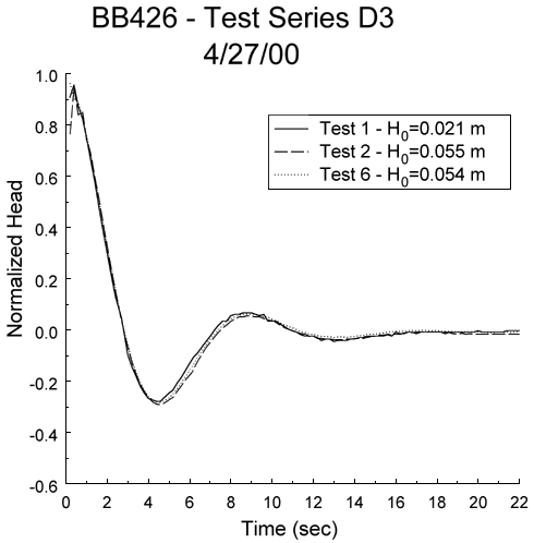
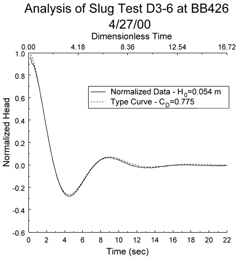
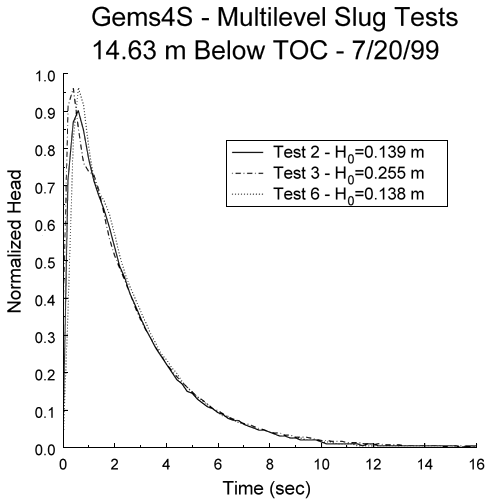
Figure 7a. Normalized head versus time plot for three slug tests performed in a monitoring well at the Geohydrologic Experimental and Monitoring Site near Lawrence, Kansas.
Butler, J.J., Jr. 1997. The Design, Performance, and Analysis of Slug Tests. Boca Raton, Lewis Publishers.
Butler, J.J., Jr., J.M. Healey, G. W. McCall, E.J. Garnett, and S.P. Loheide. Hydraulic tests with direct-push equipment. Ground Water. in review.
Butler, J.J., Jr., C.D. McElwee, and W.Z. Liu. 1996. Improving the reliability of parameter estimates obtained from slug tests. Ground Water 34, no. 3: 480-490.
Cooper, H.H., J.D. Bredehoeft, and I.S. Papadopulos. 1967. Response of a finite diameter well to an instantaneous charge of water. Water Resour. Res. 3, no. 1: 263-269.
Hvorslev, M.J. 1951. Time lag and soil permeability in ground-water observations. U.S. Army Corps of Engrs. Waterways Exper. Sta. Bull no. 36.
Kipp, K.L., Jr. 1985. Type curve analysis of inertial effects in the response of a well to a slug test. Water Resour. Res. 21, no. 9: 1397-1408.
MathSoft, Inc. 1996. Axum 5.0. Cambridge, Mass.
McElwee, C.D., J.J. Butler, Jr., and G.C. Bohling. 1992. Nonlinear analysis of slug tests in highly permeable aquifers using a Hvorslev-type approach. Kansas Geol. Surv. Open-File Rep. 92-39.
McElwee, C.D., and M.A. Zenner. 1998. A nonlinear model for analysis of slug-test data. Water Resour. Res. 34, no. 1: 55-66.
Microsoft, Inc. 1997. Excel 97. Redmond, Wa.
Springer, R.K., and L.W. Gelhar. 1991. Characterization of large-scale aquifer heterogeneity in glacial outwash by analysis of slug tests with oscillatory response, Cape Cod, Massachusetts, in U.S. Geol. Surv. Water Res. Invest. Rep. 91-4034:36-40.
Van der Kamp, G. 1976. Determining aquifer transmissivity by means of well response tests: The underdamped case. Water Resour. Res. 12, no. 1: 71-77.
Zlotnik, V.A. 1994. Interpretation of slug and packer tests in anisotropic aquifers. Ground Water 32, no. 5: 761-766.
Zlotnik, V.A., and V.L. McGuire. 1998. Multi-level slug tests in highly permeable formations: 1. Modification of the Springer-Gelhar (SG) model. Jour. of Hydrol. 204:271-282.
Zurbuchen, B.R., V.A. Zlotnik, and J.J. Butler, Jr. Dynamic interpretation of slug tests in highly permeable aquifers. Water Resour. Res. in press.