Kansas Geological Survey, Open-file Report 2005-29
by
P. Allen Macfarlane, Brownie Wilson, and Geoffrey Bohling
KGS Open File Report 2005-29
September 2005
A pilot project was undertaken at the behest of the Southwest Kansas Groundwater Management District 3 to assess the practical saturated thickness (PST) of the Ogallala aquifer in the Four Corners and the Southeast Stevens County areas of the District. The PST considers only the net thickness of saturated sediments that significantly contribute to well yield from the water table down to the bedrock surface and differs from the saturated thickness (ST), which is the total thickness of saturated sediments between the water table and the bedrock surface. Thus, PST provides a more accurate picture of water availability and may also provide insight into future water-level trends at the scale of an individual well. The pre-development PST fraction of ST was approximately 58% for both study areas. The average 2003-2005 PST in the Four Corners and Southeast Stevens County areas was 54% and 59%, respectively. These results are not surprising considering the observed heterogeneous nature of the Ogallala aquifer in outcrop. Average declines in PST from pre-development up through 2003-2005 are 44% and 8% in the Four Corners and Southeast Stevens Counties, respectively. Declines in PST are particularly widespread in the Four Corners area, but patchy in distribution. A three dimensional model of the relative sandyness of the Ogallala in southeast Kearny County reveals that sandy intervals follow the bedrock lows and tend to recur vertically upward in the Ogallala sequence. Recurrence suggests localization of the drainage within well-defined belts during thee deposition of Ogallala sediments.
The sediments above the bedrock surface are highly heterogeneous mixtures of clay, silt, sand, and gravel with many calcium-carbonate-cemented and caliche-bearing zones. Frye et al. (1956) described the Ogallala of northwest Kansas as being "homogeneous in its heterogeneity."
Saturated thickness is defined as the length of the interval between the water table and the bedrock surface as depicted in the 2004 bedrock surface elevation map (Macfarlane and Wilson, in review) at a specified time.
Practical saturated thickness (PST) is defined as the total thickness of saturated strata that significantly contribute to well yield from the water table down to the bedrock surface. Within the Ogallala, sand and sand and gravel are the permeable lithologies capable of storing and transmitting significant amounts of water to pumping wells.
Saturated thickness (ST) includes in the total thickness the saturated, low-permeability strata that do not directly transmit or contribute water to the yield of the well. Low permeability lithologies include silt, clay, shale, caliche, and calcium carbonate-cemented sands and gravels. The permeability of fine-grained sediment can be several orders of magnitude or more lower than the permeability of sand and sand and gravel. Cemented sands and caliche are included in this group because the cementation may drastically lower both bulk porosity and permeability of what otherwise would be a productive zone in the Ogallala aquifer. PST is thus a corrected, and more realistic estimate of the water immediately available to pumping wells.
The data used to estimate PST are the logs produced by (1) water-well drilling contractors and submitted on WWC-5 forms to the Kansas Department of Health and Environment and (2) Kansas Geological Survey (KGS) scientists for the county bulletins. The logs used in this study pertain only to wells where the drilled borehole for the well penetrated the bedrock surface. More than 90% of the 207 logs selected from the Four Corners study area were for wells drilled by Minter-Wilson or Henkle Drilling & Supply. In the Southeast Stevens County study area, the 48 logs used were generated by a number of different water-well drilling contractors, including Minter-Wilson and Henkle Drilling & Supply.
Descriptions of the drill cuttings provided in the WWC-5 logs and the KGS sample logs are highly individualized and reflect the individual's observational skills in describing the extremely diverse assemblage of cuttings that return to the surface during drilling. On some of the driller's logs only the primary component of the cuttings encountered for each depth interval is mentioned and none of the minor constituents represented in the cuttings are mentioned. Often the individual intervals described in these logs are short in an attempt to capture as much detail as possible. Other drillers characteristically provide only a list of the constituents types represented in the well cuttings for each depth interval or may provide some qualifications with respect to the relative proportions of each constituent present. The length of each interval described in the logs may be set arbitrarily or may coincide with distinct vertical lithologic changes, such as from clay to sand and gravel.
The bedrock surface elevation for each well location described on the WWC-5 forms was taken from the 2004 bedrock surface elevation map (Macfarlane and Wilson, in review). The pre-development and 2004 water table elevation at each well site was estimated by interpolation from the Jurachek and Hansen (1995) pre-development water-table coverage and from the 2004 elevation of the water table in the High Plains aquifer map (Kansas Geological Survey, 2005. Water Information Storage and Retrieval database [WIZARD] data available on the Internet, accessed April 20, 2005 at http://www.kgs.ku.edu/Magellan/WaterLevels/index.html).
Geologic intrpretation of the logs required a consistent means to (1) translate the driller's descriptions into lithologic descriptions and (2) quantify the relative proportions of each lithology where more than one lithology was mentioned. Rules based on the phrasing of the lithologic description were formulated to translate the interpreted descriptions into relative proportions of each lithology (clay/silt, sand, and sand & gravel) represented within each interval (Table 1). These rules were formulated based on the author's experience with interpretation of drill cuttings in the field and in some cases, based on reasonable but arbitrarily set rules. Seni (1980) adopted a similar approach using driller's logs for regional lithofacies mapping in the Ogallala in Texas. The total thickness of permeable sediment for each described interval could then be determined from the proportion of permeable sediments (sand and sand and gravel) in the interval and the interval thickness.
Table 1. Rules used to translate driller's log descriptions of drill cuttings into estimates of PST.
| Lithology/Phrasing of the Description | Percentage of the Interval Contributing to Saturated Thickness/Quantitative≅ Interpretation of Lithology |
|---|---|
| Clayey sand | 70% Contributing |
| Sandy clay | 30% Contributing |
| Sand or sand and gravel | 100% Contributing |
| Brown rock, silt, clay, shale, caliche, or cemented sandstone | Non-contributing |
| A with a lens, streak or thin strips of B | 80% A and 20% B |
| A with B | 90% A and 10% B |
| A and B or A, B (as a list) | 60% A and 40% B |
| A, B, C (as a list) | 50% A, 30% B, and 20% C |
| A, B, C, D, ( (as a list) | 40% A, 25% B, 20% C, and 15% D |
The following is an example of how this approach is applied to estimate PST for a particular interval on a driller's log with multiple entries for a single interval.
| Depth Below Surface | Driller's Description |
|---|---|
| 300 feet to 325 feet | Sand, sandy clay, clay, and caliche |
Total thickness of the interval is 25 feet. Translation of this entry into a practical saturated thickness value is covered by the rule listed at the bottom of Table 1. Sand is item A, sandy clay, B; clay, C; and caliche, D.
PST = 25[(0.4)(1.0) + (0.25)(0.3) + (0.2)(0) + (0.15)(0)] Eqn. 1
PST = 11.875 feet ≅ 12 feet Eqn. 2
In Eqn. 1, sand accounts for 40% of the interval, sandy clay, 25%; clay, 20%; and caliche ,15%. The 1.0 multiplier in the first term indicates that the entire sand thickness contributes to PST. The sandy clay is assumed to consist of 30% sand, all of which contributes to the total practical saturated thickness (multiplier of 0.3). No contribution to practical saturated thickness is made by either the clay or caliche lithologies (multiplier of 0). The total PST for this interval is approximately 12 feet or slightly less than 50% of the total interval thickness.
The total PST for the Ogallala at a particular well site is the sum of the interval PSTs between the water table and the bedrock surface at the base of the aquifer.
Each well site was spatial referenced into a Geographic Information System (GIS) based on the public land survey system legal description using the KGS LEO program (available at the Data Access and Support Center, http://www.kansasgis.org/). LEO converts township, range, section and qualifier information, either quarters or footages from a section corner, into latitude and longitude values representing the center of the smallest qualifier. Once in the GIS, the interpolated depth to water for pre-development and the average 2003-2005 time periods can readily be assigned to each well.
Using an automated procedure, the depth to water for any given time period is located within the lithologic intervals. The PST is then calculated for that time period by applying the multiplier of the interval's contribution of permeability to the difference of the water table and the bottom depth of the interval. The process is systematically repeated as it moves down the lithologic column until it reaches the bedrock depth.
The Environmental System Research Institute's TOPOGRID interpolation routine was applied to the GIS well data set to identify spatial patterns in PST variation, the PST fraction of ST, and change in PST from pre-development as both actual and percent change.
To better understand the mapped distributions of PST and PST fraction of ST, data were selected from 51 logs to portray the 3-D variation in PST in an 18.75 square mile area in the eastern part of T. 26 S., R. 36 W., Kearny County. This part of the Four Corners study area was selected because of its relatively high density of data points and the high log quality. The data were input into Rockworks 2004 " to generate a 3-D model of the Ogallala "sand" (sand and sand and gravel) content from the pre-development water table down to bedrock. The model was computed using the inverse distance anisotropic modeling method in combination with a high fidelity filter (Rockware, 2004).
The Data Sets in the Aggregate
The estimated mean and median values of PST as a fraction of the pre-development ST are approximately 58% and the distribution of the PST fraction values has lower variability in the Four Corners area than in the Southeast Stevens county area (Table 2, Figure 1). The mean PST value in the Four Corners study area is slightly more than half the mean value in the Southeast Stevens County study area. The much higher PST standard deviation in the Southeast Stevens County area indicates greater variability in the data from this area than in the data from the Four Corners area (Table 2).
Table 2. Summary statistics for the pre-development PST and the PST fraction of ST for the Four Corners and Southeast Stevens County study areas.
| Statistical Parameter | Four Corners | SE Stevens County |
|---|---|---|
| PST (feet) | ||
| Maximum | 334 | 468 |
| Minimum | 66 | 98 |
| Mean | 188 | 304 |
| Standard Deviation | 41 | 102 |
| Median | 188 | 316 |
| PST fraction of ST (%) | ||
| Maximum | 97 | 90 |
| Minimum | 17 | 20 |
| Mean | 59 | 57 |
| Standard Deviation | 13 | 19 |
| Median | 58 | 59 |
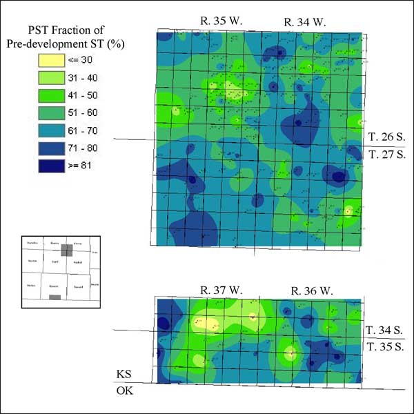
Figure 1. PST fraction of ST for the pre-development condition in the Four Corners and Southeast Stevens County study areas.
For the 2003-2005 PST fraction of ST values the estimated mean and median of the distribution are nearly the same for both study areas, 54% for the Four Corners and 59% for the Southeast Stevens County study areas (Table 3, Figure 2). The mean PST value in feet in the Four Corners study area is significantly less than half the mean value in the Southeast Stevens County study area. The 2003-2005 PST standard deviations remain relatively unchanged.
Table 3. Summary statistics for the 2003-2005 PST and the PST fraction of ST for the Four Corners and Southeast Stevens County study areas
| Statistical Parameter | Four Corners | SE Stevens County |
|---|---|---|
| PST (feet) | ||
| Maximum | 216 | 446 |
| Minimum | 22 | 92 |
| Mean | 105 | 280 |
| Standard Deviation | 31 | 99 |
| Median | 100 | 289 |
| PST fraction of ST (%) | ||
| Maximum | 96 | 94 |
| Minimum | 8 | 18 |
| Mean | 54 | 59 |
| Standard Deviation | 13 | 21 |
| Median | 53 | 59 |
Figure 2. PST fraction of ST for 2003-2005 in the Four Corners and Southeast Stevens County study areas.
The mean 2003-2005 PST for the Four Corners study area has declined by 44% from the pre-development mean value of 188 feet to 105 feet and the range of values has decreased: 344 feet-66 feet to 216 feet-22 feet. In contrast, the mean 2003-2005 PST for the Southeast Stevens County area has only declined by 7.9% of the pre-development mean value of 304 feet. Similarly, the range of PST values has declined only slightly since pre-development: 468 feet-98 feet to 446 feet-92 feet. The PST and PST fraction of ST standard deviations remain relatively unchanged.
Data Quality
The level of detail presented in the logs produced by drillers and submitted on WWC-5 forms typically varies widely in the Southeast Stevens County study area but much less so in the Four Corners study area. The average Ogallala thickness per log entry parameter is a relative measure of the level of detail contained within a driller's log. The average interval thickness per log entry for the saturated aquifer is 59.4 ft in the Southeast Stevens County study area and 24.9 ft in the Four Corners area (Figure 3). The difference in the level of detail is mostly a function of which water-well contractors have been active and at what level within each of the study areas. More than 90% of the logs analyzed from the Four Corners study area were for wells completed by Minter-Wilson and Henkle Drilling & Supply. The level of detail presented in the logs from these contractors is comparable to that found in the test-hole logs in the KGS county bulletins. In contrast, only about 40% of the logs used in the Southeast County study were generated by these drilling contractors.
Figure 3. Variability in the level of detail presented in the WWC-5 and KGS drillers' logs in the interval from the pre-development water table to the bedrock surface. Greater detail is indicated by lower thickness per unit description values.
Figure 4 is a plot showing the PST fraction of ST for the pre-development condition vs. the level of detail presented in each log, expressed as the Ogallala thickness per log entry for the two study areas sorted by drilling contractor. The data points from the Minter-Wilson and Henkle Drilling & Supply logs are relatively consistent in level of detail and the calculated fraction of ST that is PST. However, the level of detail is lower and the PST fractions are somewhat higher in the logs prepared by the other water-well contractors.
Figure 4. PST fraction of pre-development ST vs. level of detail in the driller's log sorted by drilling contractor in the two study areas.
The Pre-development and 2003-2005 Maps
Pre-development PST and the PST fraction of ST are shown for the Four Corners and Southeast Stevens County study areas in Figures 5-6 and 7-8, respectively. In the Four Corners area the PST map shows areas of greater thickness in most of T. 26 S., R34 W.; northern T. 26 W., R. 35 W.; western T. 27 S., R. 35 W.; and eastern T. 27 S., R. 34 W. An area of low PST values covers most of the southern part of T. 26 S., R. 35 W., and in a narrow band from northwestern to southeastern T. 27 S., R. 34 W (Figure 5). In the Southeastern Stevens County study area, higher PST values trend southeastward from Section 30, T. 34 S., R. 36 W. to Section 36, T. 35 S., R. 36 W.; northeastern T. 35 S., R. 37 W.; southwestern T. 34 S., R. 37 W.; and extreme northwestern T. 35 S., R. 37 S. Lower values of PST can be found in an arcuate band that extends from Secs. 8-9, T. 35. S., R. 37 W. to Sec. 8, T. 35 S., R. 36 W. (Figure 5). The maps of PST fraction of pre-development ST for both areas generally reflect the PST distribution with areas of higher and lower percentages generally corresponding to areas higher and lower thickness values (Figure 6).
Figure 5. Pre-development PST for the Four Corners and Southeast Stevens County study areas. A larger version of this figure is available.
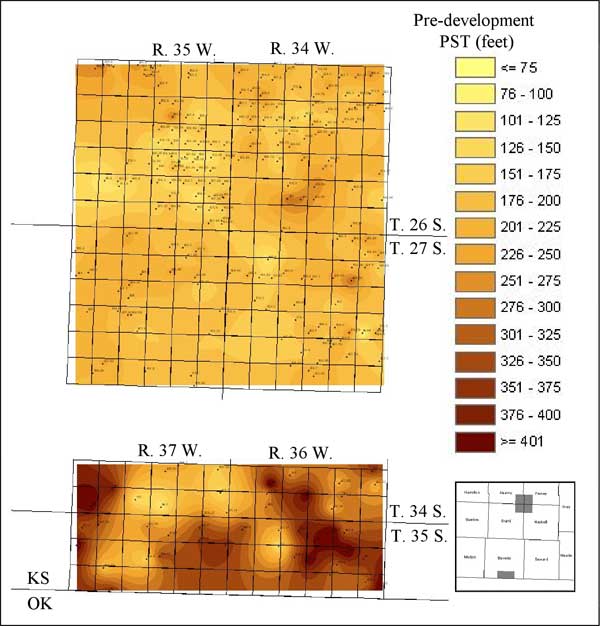
Figure 6. The PST fraction of ST under the pre-development condition in the Four Corners and Southeast Stevens County study areas. A larger version of this figure is available.
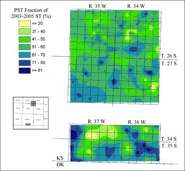
The overall pattern of highs and lows observed in the pre-development maps of PST and the PST fraction of ST are apparent in the 2003-2005 maps for the Four Corners and in the Southeastern Stevens County area maps (Figures 7 and 8). In the Four Corners area, lighter brown shades on the 2003-2005 PST map contrast with the darker brown color bands in pre-development PST, indicating significant overall reduction. In contrast, the pattern of darker and lighter browns on the both PST maps of the Southeast Stevens County indicate little, if any, change. Table 3 lists the summary statistics on the change in PST from pre-development to 2003-2005.
Figure 7. 2003-2005 PST for the Four Corners and Southeast Stevens County study areas. A larger version of this figure is available.
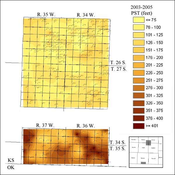
Figure 8. The 2003-2005 PST fraction of ST in the Four Corners and Southeast Stevens County study areas. A larger version of this figure is available.
Changes in PST from Pre-development to 2003-2005
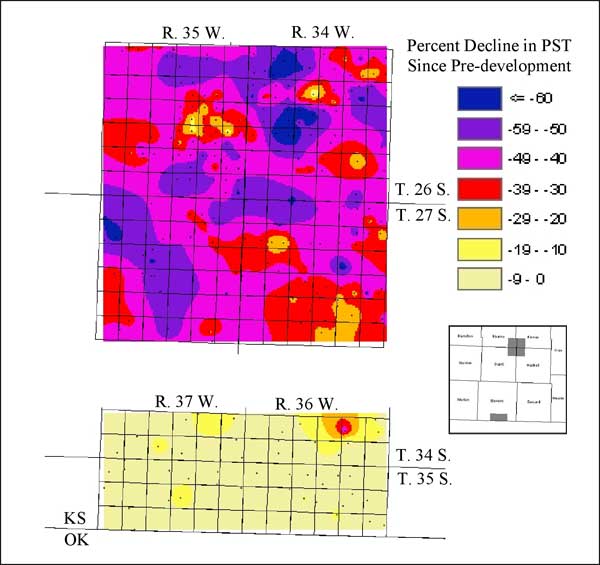
The aggregate statistical data in Table 4 show that the PST decline has been much greater in the Four Corners than in Southeast Stevens County study areas. Since pre-development approximately 80 feet or 44% of the pre-development PST on average has been removed from the Ogallala aquifer in the Four Corners area compared to approximately 20 feet of decline or less than 10% of the pre-development PST on average in the Southeast Stevens County area. Figures 9 and 10 show that the loss of PST since pre-development is patchy and widespread across the Four Corners study area, but is more localized in Southeast Stevens County.Table 4. Change in PST and PST fraction of ST (pre-development minus the 2003-2005 values) in the Four Corners and Southeast Stevens County study areas.
| Statistical Parameter | Four Corners | SE Stevens County |
|---|---|---|
| Change in PST (feet) | ||
| Maximum | 174 | 112 |
| Minimum | 2 | 0 |
| Mean | 83 | 24 |
| Standard Deviation | 30 | 17 |
| Median | 85 | 20 |
| Change in PST Fraction (%) | ||
| Maximum | 77 | 50 |
| Minimum | 2 | 0 |
| Mean | 44 | 8 |
| Standard Deviation | 13 | 7 |
| Median | 44 | 7 |
Figure 9. Decline of PST since pre-development in the Four Corners and Southeast Stevens County study areas. A larger version of this figure is available.
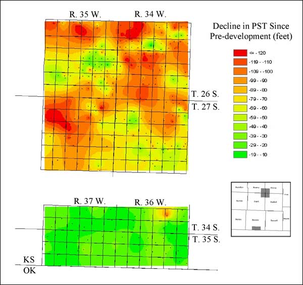
Figure 10. Percent decline in PST since pre-development in the Four Corners and Southeast Stevens County study areas. A larger version of this figure is available.
Taking Into Account Data Quality in the Southeast Stevens County Study Area
The level of detail in the drillers' descriptions of the Ogallala is much less uniform in Southeast Stevens County than in the Four Corners area (Figure 3). The calculated PSTs for those less detailed Southeast Stevens County logs tend to be higher than for the logs where the detail is greater (Figure 4).
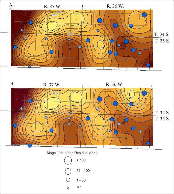
The variable quality of the southeast Stevens County PST data suggests that it may be more reasonable to use a smoothing interpolator, rather than an exact interpolator, to produce a map of PST in this area. An exact interpolator (such as inverse-distance-squared interpolation or kriging) will exactly reproduce the input data values at well locations, forcing the mapped surface to honor the well data, even when the data values at the wells are subject to uncertainty, as they are in this case. A smoothing spline interpolator, on the other hand, produces a smoother surface that more broadly represents the data trends, without forcing the mapped surface to exactly match the data values at the wells. The smoothing spline surface is fit to the observed data using a regression procedure which aims to minimize the sum squared error between observed and predicted data (PST) values at the wells while simultaneously minimizing the overall curvature or roughness of the fitted surface (Hastie et al., 2001). In general, smoother surfaces produce greater mismatches between observed and predicted data values, and vice versa. The tradeoff between smoothness and data fit is controlled by a smoothing parameter. The smoothing spline function employed in this study is that included in the mgcv package developed by Wood (2000, 2003) for the R statistical language (Ihaka and Gentleman, 1996; http://www.r-project.org). This function uses a cross-validation procedure to estimate a smoothing parameter that yields an optimal balance between smoothness and data fit.
In addition, the smoothing spline fitting function allows the inclusion of variable weights on the residuals at the data points (wells). In this study, we have developed two different maps of the PST in southeastern Stevens County, one with the PST values at all wells weighted equally (or, one might say, with no weighting), and the other with each PST value weighted inversely to the thickness per log entry at that well, so that PST values developed from more detailed logs are weighted more heavily than those developed from less detailed logs. The map with variable weighting is shown in Figure 11a and that with equal (or no) weighting is shown in Figure 11b.
Figure 11. The effect of smoothing using splines with weighting (A) and splines without weighting (B). The size of the blue dot represents the magnitude of the error induced from using the smoothing of the raw data. A larger version of this figure is available.
Ogallala Aquifer Framework in T. 26 S., R. 36 W.
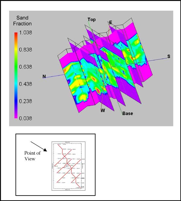
Figures 12-13 and Figures 14-15 present different views of the three-dimensional model of and the accompanying fence diagram through the pre-development saturated Ogallala aquifer in T. 26 S., R. 36 W. The model upper and lower boundaries are the pre-development water-table and the bedrock surface, respectively, and are displayed as pink upper and lower boundaries (sand fraction = 0). Blue to purple intervals between the pre-development water table and the bedrock surface are dominated by clay, silt, and caliche and intervals in red and yellow by sand or sand and gravel. The illustrations show that intervals dominated by the coarser grained sediments in the lower part of the aquifer are associated with fluvial channels that have been incised into the bedrock and is also true for most of the sand bodies higher up in the saturated Ogallala. This recurrence of sands up through the saturated Ogallala suggests a drainage that shifted back and forth over time across a corridor of limited extent. Comparison of the pre-development PST maps with the different views of the three-dimensional model suggests that the linear band of higher PST that crosses from Kearny into Haskell county can be attributed to a stacking of the fluvial channel sands within the Ogallala. Lenses of clay, silt, and caliche are locally extensive and scattered vertically and laterally through the section. The illustrations also show that the sandy areas are interconnected by less sandy deposits (on the order of 60% "sand"). This indicates good lateral but apparently limited vertical hydraulic connection between vertically adjacent permeable zones within the aquifer.
Figure 12. Three-dimensional model of the "sand" fraction in the pre-development saturated part of the Ogallala aquifer in T. 26 S., R. 36 W. as viewed from the east-southeast.
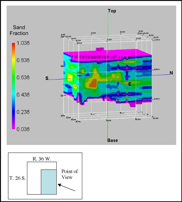
Figure 13. Three-dimensional model of the "sand" fraction in the pre-development saturated part of the Ogallala aquifer in T. 26 S., R. 36 W. as viewed from the northwest.
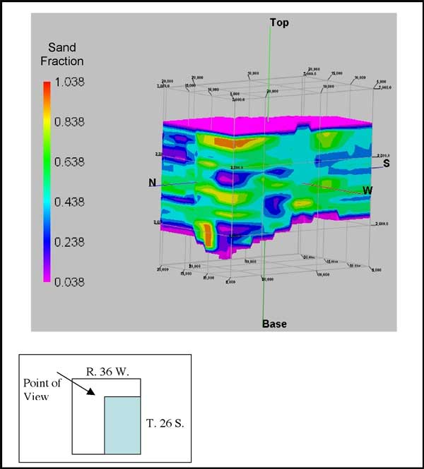
Figure 14. Fence diagram through the three-dimensional model of the "sand" fraction in the pre-development saturated Ogallala in T. 26 S., R. 36 W. as viewed from above at a vantage point northeast of the modeled region.
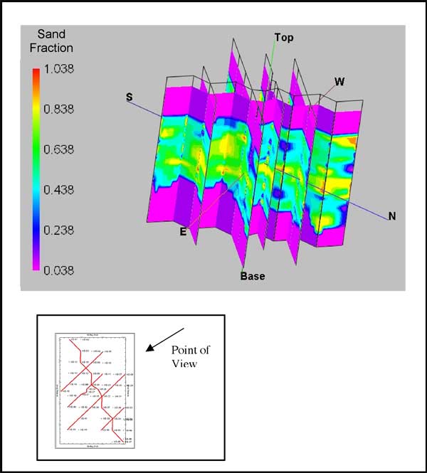
Figure 15. Fence diagram through the three-dimensional model of the "sand" fraction in the pre-development saturated Ogallala in T. 26 S., R. 36 W. as viewed from above at a vantage point northwest of the modeled region.
The PST Concept
PST is a useful concept for characterizing water availability in aquifers that display a high degree of heterogeneity (such as the Ogallala), because this parameter represents the net thickness of permeable water-saturated sediments. PST may also provide a qualitative assessment of how the aquifer should function under pumping conditions at the scale of an individual well. The highly permeable coarser-grained fraction directly provides water to pumping wells, whereas the finer-grained or the cemented low-permeability fraction slowly releases water as leakage or delayed drainage to the coarser grained zones. Thus, in areas of the aquifer where the net thickness of permeable sediments is low in relation to total thickness, the water saturated non-aquifer fraction may act to buffer depletion of the resource in the long term by slow leakage of water to the coarser-grained fraction.
The impact of interbedding of high and low permeability layers on aquifer functioning since pre-development can be seen locally on some hydrographs of wells within both study areas. The best example is the hydrograph of a well in the NENESE Sec. 28, T. 27 S., R. 34 W. (Figure 16). Included on the graph is the vertical distribution of the "sand" fraction (sand plus sand and gravel) in the Ogallala at that location from the pre-development water table down to bedrock interpreted from the driller's log of the well. The hydrograph shows the unsteady decline of the water table across a sequence of interbedded "sandy" to non-"sandy" zones in the upper part of the Ogallala. Note that the decline rate abruptly changes as the water table moves across the boundaries between zones. As the water level passes across the top of a non-"sandy" zone, the decline rate tends to accelerate. At or near the lower boundary between the non-"sandy" and the underlying "sandy" zone, the water level decline rate slows and later increases. This behavior can be explained by considering the contrasting water-yielding characteristics of the "sandy" and non-"sandy" zones, which are primarily silt and clay. Because of their low permeability and high storage capacity, silt and clay do not yield water significant amounts of water directly to wells during the pumping season. Locally, these layers may also act to partially confine underlying aquifer zones. Hence, the water table declines more rapidly across these layers. Once the water table declines below these layers, the "sandy" layer is no longer under partial confinement and delayed drainage from the overlying non-"sandy" zone acts to lower the water- level decline rate. This behavior of the declining water table suggests that significant amounts of water may be slowly released from storage in areas where the PST fraction is low and may act to extend the usable lifetime of the aquifer.
Figure 16. The water-level hydrograph and the vertical distribution of "sandy" zones within the Ogallala aquifer at NENESE Sec. 28, T. 27 S., R. 34 W. in Haskell County. Note the changes in the rate of decline of the water level in the vicinity of the boundaries between zones of differing "sand" content in the Ogallala aquifer within the blue ellipse.
Methodology Uncertainty
The methodology used to calculate PST is deceptively simple, but uncertainty in the results is difficult to assess. The factors contributing to uncertainty include, (1) the driller's knowledge level and ability to observe and describe the cuttings produced during the drilling, and to conceptualize the subsurface based on appearance and disappearance of lithologies in the cuttings; and (2) the analyst's ability to recast the narrative portion of the driller's log in geologic terms. To some extent the first factor can be taken into account by selecting logs produced by drilling companies known for producing good quality data and by noting the level of descriptive detail in the log. The second factor is more difficult to control because the manner in which cuttings are described typically varies from one driller to the next even within the same company. Thus, the analyst must be able to interpret the terms used by drillers and rely on the consistent application of a set of rules based on how the driller might describe the cuttings and enter observations on the log. Using these rules, it is possible to calculate the lithologic composition of the Ogallala and the total thickness of permeable sediments (sand and sand and gravel). Ideally, these rules should tested and calibrated by polling drilling contractors to see if these interpretive rules are reasonable or devised by comparing depth interval by depth interval a well-site geologist's descriptions with that of the driller. However, such field-testing was not done for this project.
Determination of PST using the WWC-5 records of wells is also a manually intensive process because the logs are not in a digital format. Two 8-hour days of effort by a professional scientist were required to process the 256 logs and create the database used in this project. Site location and elevation information are readily available in electronic format and can be quickly integrated with the logging information in the database.
Results
The low pre-development mean and wide range of PST values relative to ST in both study areas are not surprising considering the heterogeneous nature of the Ogallala aquifer. Outcrops of the Ogallala typically consist of a significant fraction of non-aquifer grade sediments, including caliche, silt and clay, and freshwater limestone. Detailed logs from recent drilling through the unsaturated zone and the upper part of the Ogallala aquifer in southwest Kansas by the USGS for the NAWQA program, reveal numerous intervals consisting entirely or mostly of silt and clay (McMahon, 2001; McMahon et al., 2003).
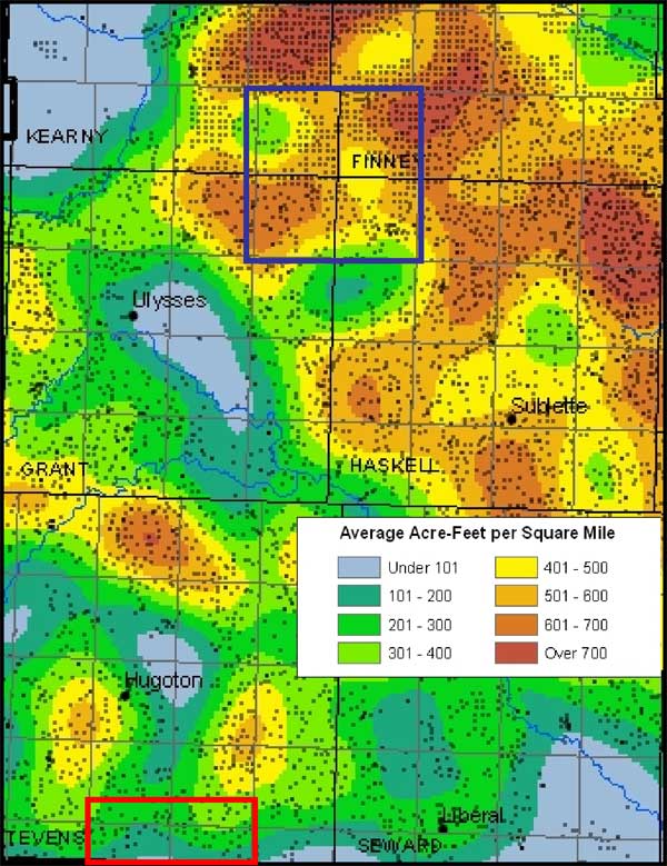
The decline in PST between pre-development and 2003-2005 and how it is distributed in both areas relative to water-use density differs between the two study areas (Figure 17). Declines in the Four Corners area are widespread and patchy in distribution with areal extents that range up to the size of a township (Figures 9 and 10). Whereas the high decline areas are much more localized on the order of a section in extent in the Southeast Stevens County area (Figures 9 and 10). Larger declines seem to correspond to high water-use density areas in the Four Corners (compare the distribution of high and low PST decline areas in Figure 9 with the high and low water use density areas in Figure 17). In the Southeast Stevens County area water-use density is much lower than in the Four Corners area and PST declines are low except in the southeastern part of T. 34 S., R. 36 W. where there is an area of higher decline (Figures 9, 10, and 17). According to the GMD manager the Southeast Stevens County area has been slow to develop because this has been considered to be an area of low well yield, presumably because of low aquifer transmissivity (Mark Rude, personal communication, 2005). However, the pre-development and the 2003-2005 PST and PST fraction maps only show localized areas where well yields might be lower.
Figure 17. Average water use density (1990-2003) in a portion of southwest Kansas using a 5-mile search radius with the Four Corners and Southeast Stevens County study areas outlined in blue and red, respectively.
In the two study areas, the pre-development net thickness of what are judged to be permeable sediments described on the drillers' logs is on the order of 50-60% of the total water saturated sediment thickness. At pre-development the mean PST thickness was 188 feet and 304 feet in the Four Corners and Southeast Stevens County study areas, respectively. By 2003-2005, the mean PST had declined to 105 feet and 280 feet in the Four Corners and Southeast Stevens County study areas, respectively. These changes represent a 44% and an 8% decline in PST in the Four Corners and Southeast Stevens County study areas, respectively.
Frye, J.C., Leonard, A.B., and Swineford, A., 1956, Stratigraphy of the Ogallala formtion (Neogene) of northern Kansas: Kansas Geological Survey, Bulletin 118, 92 p.
Hastie, T., Tibshirani, R., and Friedman, J., 2001, The Elements of Statistical Learning, Data Mining, Inference, and Prediction: Springer-Verlag, New York, 533 pp.
Ihaka, R., and Gentleman, R., 1996, R: A language for data analysis and graphics: Journal of Computational and Graphical Statistics, 5, 299-314.
Macfarlane, P.A., and Wilson, B.B., in review, Enhancement of the bedrock surface elevation map of the Ogallala portion of the High Plains aquifer, western Kansas: Submitted to the Kansas Geological Survey for publication.
McMahon, P.B., 2001, Vertical gradients in water chemistry in the central High Plains aquifer, southwestern Kansas and Oklahoma panhandle: U.S. Geological Survey, Water-Resources Investigations Report 01-4028, 47 p.
McMahon, P.B., Dennehy, K.F., Michel, R.L., Sophocleous, M.A., Ellett, K.M., and Hurlbut, D.B., 2003, Water movement through thick unsaturated zones overlying the central High Plains aquifer, southwestern Kansas, 2000-2001: US Geological Survey, Water-Resources Investigations Report 03-4171, 32 p.
Seni, S.J., 1980, Sand-body geometry and depositional systems, Ogallala formation, Texas: Texas Bureau of Economic Geology Report of Investigations 105, 36 p.
Wood, S.N., 2000, Modelling and smoothing parameter estimation with multiple quadratic penalties: Journal of the Royal Statistical Society B, 62(2), 413-428.
Wood, S.N., 2003, Thin plate regression splines: Journal of the Royal Statistical Society B, 65(1), 95-114.
Kansas Geological Survey, Geohydrology
Placed online Feb. 1, 2006
Comments to webadmin@kgs.ku.edu
The URL for this page is http://www.kgs.ku.edu/Hydro/Publications/2005/OFR05_29/index.html