 , where n is the total number of
element types in the model. We fill node (i, j) using a scheme similar to
the one used in the initialization phase: We generate a random number x
between 0 and 1 (0 < x < 1), and partition the interval from 0 to 1
into n subintervals. If
  the mth subinterval has width rm, while the n-1st subinterval has
width qa and the nth subinterval has width qb. The starting point of
each subinterval m is
xm-1 and the ending point is xm, where
 for
for  ,
,
 and
and
 (and x0 = 0). The relationship
between the probabilities (qm , rm) and the intervals [xm-1, xm] is
illustrated below:

Node (i, j) is filled with element m where m is such that xm-1 < x < xm. We continue filling the lattice until all of the lattice nodes are filled.
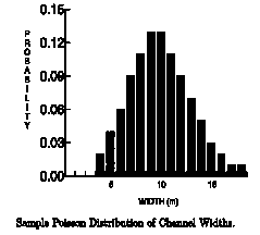
The mean size of each element is determined by field observation, and is allowed to vary according to a Poisson distribution. This means that the width and length of an element will be determined randomly, but the distribution will be weighted more heavily near their respective mean sizes. These widths are incorporated in calculating the growth probabilities qk. For example, if a channel has a mean width of 10 m then, at a given location, the probability that the channel will have a width w is shown in the illustration below:

Appendix E contains a completed run of the prototype model for the Terra Cotta strata, showing first the initialization field model and then the final output model. This model only had three distinct elements: Channel elements (Element One); foreset-macroform elements (Element Two); and lateral accretion elements (Element three). Note that the model actually assigns an element to a node and not to a region, but these nodes represent a square area, so we have colored the entire grid above and to the right of the assigned node. The model was run for only a small area, hence the small lattice size. Appendix F contains a complete printout of the C-language modeling program.
The model quickly grows to fill all of the nodes in the grid. At this time the geologist interprets the model for plausibility, and another model is generated, continuing the iterative process until we have a set of geologically plausible two dimensional models. We then add the depth and thickness dimensions, giving a final result of a set of geologically plausible, three dimensional models of a particular formation. Each model can then be stacked with models of other layers to determine an overall description of the aquifer.
Previous Page--Model generation ||
Next Page--Rocktown Channel Exposures
Dakota Home ||
Start of the Stochastic Modeling Report