The prediction of a continuous variable will be illustrated using core permeability and logging measurements from the Lower Permian Chase group in the Hugoton gas field in southwest Kansas. This represents a regression-style application, with logging measurements of the porosity and the uranium component of the spectral gamma ray log being used to explain or predict core permeabilities. Doveton (1994) examined the least squares regressions of log-permeability on different pairs of logs obtained from the well and found that the porosity-uranium pair was most effective, explaining about 41% of the total variation in the log-permeability. We will take advantage of Kipling's ability to represent nonlinear behavior and develop a model of permeability itself (rather than log-permeability) as a function of the porosity and uranium logs.
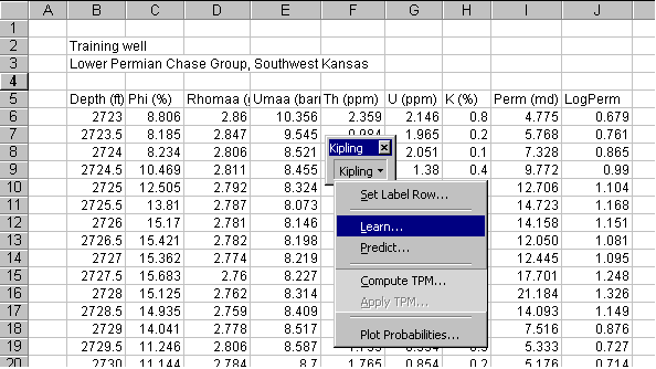
The log values and the core permeability for the training well have been gathered together in the Excel spreadsheet shown below, with each variable in a column and with variable labels in a single row. To develop a model for permeability using this data, we select Learn... from the Kipling menu as shown:

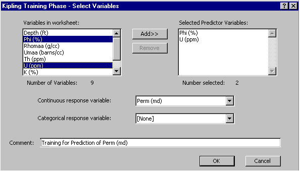
We are then presented with a dialog box asking us to specify the variables to use in the analysis. Here we have selected Phi (%) and U (ppm) as the predictor variables and Perm (md) as the continuous response variable. We have also typed in a comment to be saved on the worksheet which will contain the results of the training process:
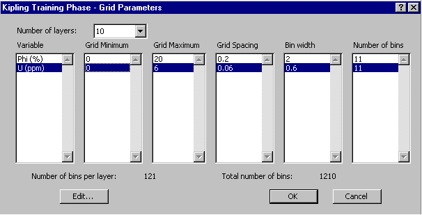
The next dialog box asks us to specify the discretization of variable space to employ in developing the model. As described in the theoretical background, the CMAC algorithm employed in Kipling algorithm involves the discretization of predictor variable space into a grid with a certain number of grid nodes along each variable axis. The specifications of this grid are given in the Grid Minimum, Grid Maximum, and Grid Spacing list box for each variable. The grid spacing along each axis determines fundamental level of resolution of the model. The data distribution and response variable behavior are represented using data counts and averages accumulated over larger bins, each encompassing the same number of grid nodes along each variable axis. Several alternative layers of bins are used, each offset from the previous layer by one grid node along each axis. The number of alternative layers is set using the Number of layers dropdown box. This together with the grid spacing determines the bin width along each variable axis. Here we have specified 101 grid nodes along both the porosity and uranium axes and have told the software to use 10 alternative layers of averaging bins:
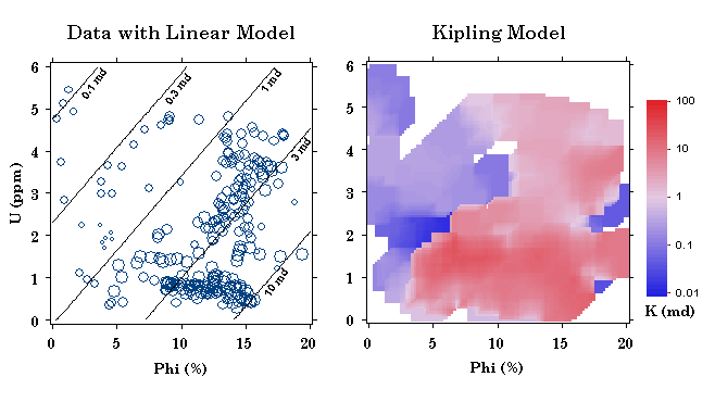
The output from the learning process is termed a "histogram" worksheet. The information in this worksheet, including data counts and response variable averages in each bin, represents the model developed by the learning process. The model we have just developed can be used to predict permeability for porosity-uranium value pairs that are sufficiently close to those contained in the training dataset. Predicting over a grid of porosity and uranium values shows the overall shape of the Kipling model for permeability as a function of porosity and uranium, shown on the right below. The plot on the left shows the original data values, with the circles scaled according the logarithms of the permeability values, together with contours representing the linear regression model of log-permeability versus porosity and uranium. The linear regression model captures a general trend of increasing permeability with increasing porosity and decreasing uranium, but fails to capture important features like the cluster of very low permeability values in the vicinity of (Phi = 5%, U = 2 ppm). The Kipling model captures quite a bit of the local detail while also providing some degree of generalization from the training data.
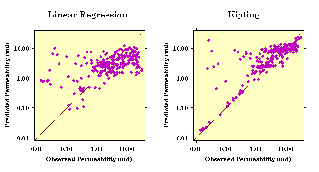
Crossplots of the actual and predicted permeabilities for the two models show Kipling's improved reproduction of the training data:
As with neural networks, it is quite possible to "overtrain" Kipling, forcing it to reproduce the details of the training data too closely. The resulting loss of generalization almost invariably decreases the accuracy of predictions based on data other than that used in training. Cross-validation studies are probably the most effective means for establishing a proper balance between generalization and reproduction of detail.
Previous Page--Theoretical Background ||
Kipling Home || Next
Page--Categorical Example