Original published in D.F. Merriam, ed., 1964, Symposium on cyclic sedimentation: Kansas Geological Survey, Bulletin 169, pp. 399-413

Finding the Ideal Cyclothem

by William C. Pearn

Kansas State University, Manhattan, Kansas

Abstract

Rock sequences can be translated into numerical sequences by associating with each recognized lithology an integer (1 to 5) according to a fixed classification scheme. Finite numerical sequences, corresponding to actual measured sections, can then be compared to infinite numerical sequences, corresponding to ideal cyclothemic repetitions. If an actual sequeuce is considered to be a fragmentary ideal, with some lithologies missing owing either to nondeposition or subsequent removal, the deviation of the actual from the ideal can be measured by a discordonce index defined as the minimum value of the number of missing lithologies. The ideal sequence which best explains the over-all characteristics of a sample of finite sequences is the ideal for which the average value of the discordance index is least.

In this manner, the "best" ideal cyclothem for an area and stratigraphic interval of interest can be determined from arithmetic operations on a sample of actual rock sequences derived from measured sections within the area and interval. The method is developed, and application is made to measured sections from the Missourian-Wolfcampian (Upper Pennsylvanian-Lower Permian) interval of northeastern Kansas.

Of particular interest is the ideal sequence which corresponds to the ideal cyclothem proposed by R. C. Moore for this region. Results indicate that the best ideal cyclothem for the area-interval considered would be similar to that proposed by Moore. However, the classification used was clearly inadequate and some deficiencies of the classification are discussed hriefly.

Introduction

The general repetitive nature of Pennsylvanian and Permian rock sequences is well known and is particularly striking in parts of the Midcontinent region. It seems that the concept of cyclic sedimentation is well established, at least within this region and stratigraphic interval.

Throughout geologic history epicontinental seas have repeatedly inundated the present land masses. In virtually every locality where a sedimentary sequence exists, it contains a record of the transgressions and regressions of such seas. It is natural to equate depositional cycles with marine oscillations. However, the large number of oscillations seemingly required for deposition of the Pennsylvanian cyclothems has led to speculation that physical transgression and regression may not have been involved in each individual "cycle." The terms transgression and regression as used here should be understood to stand symbolically for whatever mechanism may actually have been operative.

A portion of the investigation (Pearn, 1964) was designed to question the existence of underlying mechanisms governing the nature of repetitive sedimentary sequences. It may be assumed with confidence that such mechanisms exist. Speculation concerning the nature of these mechanisms is interesting, but conclusions are difficult if not impossible to prove. More practical questions concern the nature of the repetitive record itself. For instance, in a given region and within a given stratigraphic interval, what lithologic units constitute the ideal cyclothem? What sequence, if any, is repeatedly though imperfectly represented by actual rock sequences?

A well-known ideal cyclothem, which seems to be applicable to Pennsylvanian rocks in Kansas, is that proposed by R. C. Moore (1936). Recognition of an ideal cyclothem has been possible only after the study of large numbers of actual rock sequences. The process is inductive. From an essentially infinite number of possible ideals one is selected which seems to fit the observational data at least as well as any other.

If the selected ideal cyclothem implies a reasonable transgressive-regressive mechanism, as is certainly true of the Moore ideal, then the over-all concept takes on additional weight as a unifying hypothesis. A recognized ideal cyclothem has the attributes of a "natural law" in the sense that it helps to organize diverse observational data in terms of a single, simple, and reasonable hypothesis. An ideal cyclothem is not only scientifically useful but intellectually satisfying.

The purpose of this investigation was to provide the operational mechanics of an objective procedure for making the necessary inductive step in the recognition of an ideal cyclothem. The methods used were specifically designed to answer certain questions about cyclothems in Kansas. Some of the procedural details, especially of classification and sampling, were dictated by expedience and tailored to use available data. Refinements and improvements will be necessary. It is hoped, however, that the general approach used here will prove useful in future studies and other areas.

Acknowledgments--The author wishes to thank Dr. Leslie Marcus, Department of Statistics, Kansas State University, for help and advice; Dr. E. J. Zeller, Department of Geology, The University of Kansas, for the suggestion that questions about cyclothems might be handled by considering numerical sequences; and Dr. D. F. Merriam, Kansas Geological Survey, for invaluable service both in supplying the data and in making available computer facilities.

Appreciation is expressed to the Computation Centers at both Kansas State University, where the IBM 1620 and IBM 1410 computers were utilized, and The University of Kansas, where the IBM 1620 was used.

Simplifying the Moore Ideal Cyclothem

How well does the Moore ideal cyclothem describe rock sequences within the stratigraphic range for which it was intended? With this general question in mind, the first step was to formulate the Moore ideal as a numerical sequence. Moore's original numerical designations were easily adapted (see Table 1).

Table 1--Revised designations for cyclothem units (after Moore, 1936, p. 24-25).

The reason for combining the shales .1 and .2 into a single lithologic unit, 2, was merely that the first criterion in classification was to be gross lithology. It was desirable, in so far as possible, to restrict the application of other criteria such as fossil content and the presence or absence of coal. Similarly, the regressive units, .6, .7, .8, .9, would have been difficult to distinguish from their transgressive counterparts, .1, .2, .3, .4, except on the basis of relatively subtle distinctions. For that reason, corresponding transgressive and regressive units were considered equivalent. With these modifications the Moore ideal cyclothem is expressible as: ...1 2 3 4 5 4 3 2 1 2 3 4 5 4 3 2 1 2 3 4 5 4 3... an infinite sequence consisting of adjacent transgressive (1 2 3 4 5) and regressive (5 4 3 2 1) hemicycles. The units 1 and 5 are at once both transgressive and regressive and will here be called pivotal lithologies. Moore (1936, p. 26) anticipated the consideration of such an infinite sequence when he remarked:

The entire cyclothem thus records a single marine pulsation. ...This nearly symmetrical or harmonic sort of rhythm might be expressed numerically by the sequence 0-1-2-3-4-5-4-3-2-1-0.

In order to complete the classification, it was necessary to consider additional criteria. Specifically, it was necessary to distinguish between the shales, 2 and 4, and between the limestones, 3 and 5. The scheme shown in Table 2 was adopted. The primary criteria correspond to Moore's original descriptions.

Table 2--Criteria for the distinction between nonsandstones.

If the chief purpose of this investigation were to establish, once and for all, the "best" ideal cyclothem for the area considered, the classification of Table 2 would have to be considered inadequate. The investigation purports to be objective, yet the classification contains many snbjective elements. Still worse, the ultimate appeal to "position" when decision seems hopeless assumes the underlying Moore ideal, and to answer questions about the Moore ideal on this basis is decidedly circular.

Classification, however, may be considered a separate problem. The purpose of this investigation is not to arrive at unshakeable conclusions, bnt rather to indicate a line of attack which should lead to objective conclusions, given a better classification, more detailed data, and so forth.

The Discordance Index, G

The second step in the procedure was to define a numerical statistic to serve as a mea. sure of the amount of deviation of any actual rock sequence from the Moore (or some other) ideal sequence. For this purpose, the discordance index G was defined as follows:

1. Observe the first lithologic unit, a₁ (a₁ = 1, . . ., 5) of the finite sequence of interest.
2. Consider a portion of the ideal sequence beginning with a₁ and such that a₁ occurs within a transgressive hemicycle.
3. Sum the number of lithologic units which would have to be inserted to couvert the observed sequence of (1) to the ideal sequence of (2). Call this sum G₁.
4. Consider a portion of the ideal sequeuce beginning with a₁ and such that a₁ occurs within a regressive hemicycle.
5. Sum as in (3), but comparing the observed sequence of (1) with the ideal sequence of (4). Call this sum G₂.
6. The statistic G, characteristic of the observed sequence of interest and the ideal being considered. is the minimum of G₁ and G₂.

G = min (G₁, G₂)

This definition will, perhaps, be clarified by an example. Consider a seven-unit actual sequeuce as follows:

actual sequence, 2 3 2 5 3 2 1
ideal (transgressive), . . . 2 3 4 5 4 3 2 1 2 3 4 5 4 3 2 1. . .
sum of omitted units, 4 + 4 + 1 = 9 = G₁
ideal (regressive), . . . 2 1 2 3 4 5 4 3 2 1 2 3 4 5 4 3 2 1. . .
sum of omitted units. 2 + 4 + 4 + 1 = 11 = G₂

G = min (G₁, G₂) = G₁ = 9

The statistic G is called the discordance index because it represents the number of omissions from the observed sequence if the ideal is really applicable. The larger the value of G, the less likely it seems that the observed sequence actually resulted from the transgressive-regressive repetitions implied by the ideal. Because equivalent lithologies in the transgressive and regressive hemicycles are considered indistinguishable, it is logical to characterize the observed sequence by the choice of initial transgression or regression which minimizes G. In this way, the ideal sequence being considered is given the "benefit of the doubt."

Clearly, the discordance index so defined was not the only possible choice for a measure of observed deviation from ideal sequences. The investigation reported here rests on the assumption that G was a natural and interesting choice. The method. used, however, would be adaptable to other statistics, and this is a possible direction for future investigation.

Formulating the Questions

The general question which guided the translation of the Moore ideal into a numerical sequence and the definition of the discordance index must be made more specific. It can be rephrased in the following alternative forms:

QUESTION A.
1. How well does the Moore ideal cyclothem describe the rock sequences summarized as the composite section of the Kansas rock column?
2. Would some other ideal sequence describe these "facts" better?

QUESTION B.
1. How well does the Moore ideal cyclothem describe actual rock sequences observed in outcrops reported from Kansas localities?
2. Would some other ideal sequence describe actual rock sequences better?
3. Is there adequate reason to believe that actual rock sequences are not random?

Generating the Population of Seven-unit Sequences

In order to answer the above questions, it was necessary to restrict the length of the actual sequences which would serve as data units. In particular, question B3 required that the distribution of G in a population of finite sequences be known. If the population of all possible sequences of length L were generated, the distribution of G in that population could be determined. On the assumption of equal likelihood among the sequences, the probability of occurrence of any particular G-value could also be found. The following information was desired:

(1) All permutatious of L lithologies chosen from the five recognized lithologic types such that identical lithologies do not occur in adjacent positions in sequence. This restriction was necessary because the actual sequence 1223454, for instance, would probably be reported as 123454.
(2) The values of G which result from comparing each sequence of the population with the Moore ideal.

It can easily be shown that the number of sequences in such a population is given by:

N = n (n-I)^L-1

where n is the number of distinct lithologies recognized, five in this case, and L is the length of the sequences to be generated. To see this, we may visualize the filling of L positions in sequence by n distinct kind. of items. Let a₁, a₂, . . . a_L be the items to be chosen. There are n choices for a₁ and for each of these there are n-l choices for a₂. The single restriction is a₁ ¬ a₂. For given a₁, a₂ there are n-1 choices for a₃ and so forth. In general,

a_i ¬ a_i+1 from which the above result is clear.

It was desirable to fix L in such a way that the population would be of a manageable size, while the length of actual sequences used would be sufficient to test the hypotheses of interest. Intuitively, it would not have been wise to use actual sequences of length 2, for example, to test hypotheses concerning an ideal sequence with hemicycle length 5. After preliminary considerations of this kind, L was chosen as 7 and the population consisting of

N = 5(4)⁶ = 20,480

sequences was generated. At the same time each G was calculated. Table 3 shows the distribution of G in this population. If the sequences of the population are equally likely to occur in nature, then each possible value of G (0, 1, . . ., 18) will have the probability shown in column 3. In other words, Table 3 gives the expected frequencies of occurrence for each possible G-value under the hypothesis of random deviation from the Moore ideal.

Table 3--Distribution of G in the population of seven-unit sequences based on the Moore ideal.

A Population of Alternative Ideals

Would some other ideal sequence describe the facts better? It was necessary to ask in turn, what other ideal sequences are possible? Any sequence which contains each of the recognized lithologies at least once could be taken as an ideal hemicycle. Some sequences such as 1 2 3 2 3 2 3 4 3 2 3 2 3 2 3 2 3 2 3 4 5 4 do not seem reasonable in terms of the complexity of the transgressive-regressive mechanism implied if such a sequence were to be considered a hemicycle. Nevertheless, there is no limit to the number of sequences which might improve upon the Moore ideal cyclothem. In order to search systematically for the "best" ideal sequence, it was necessary to restrict the universe of ideals in some manner.

Because the population of seven-unit sequences was already available, it was convenient to consider a set of ideal hemicycles obtained by examining each sequence of the larger population to see whether either the 5th or 6th positions could be considered pivotal. The procedure was:

1. Designate the lithologies in each sequence as a₁, a₂, . . ., a₇ where the suhscripts indicate the position in sequence. Then a₁ = k (i=1...7; and k=1...5).
2. If the set consisting of a₁, a₂, . . ., a₅ contains each integer (1,2, . . ., 5) exactly once, i.e. the first five lithologies are all different, then the sequence is a potential ideal generator subject to satisfaction of the restriction in (3). If the set consisting of a₁, a₂, . . ., a₆ contains each integer (I, 2, . . ., 5) at least once, i. e. exactly one lithology is repeated among the first six, then the sequence is a potential ideal generator subject to satisfaction of the restriction of (4).
3. If a₄ = a₆ and a₃ = a₇ then the sequence is pivotal around a₅ and tbe hemicycle length is 5.
4. If a₅ = a₇ then the sequence is pivotal around a₆ and the hemicycle length is 6.

For example, consider the sequence 3 2 4 1 5 3 5. Among the first five lithologies, all are represented. However, a₄ ¬ a₆ (1 ¬ 3), so that the sequence is not pivotal around a₅. Among the first six lithologies, exactly one lithology (3) is repeated, and a₅ = a₇ = 5. The sequence is pivotal around a₆, and a₁, a₂, . . ., a₆ constitute an ideal hemicycle.

The population of hemicycles obtained in this manner has 1200 members. From these hemicycles 660 distinct ideal sequences can be generated. Consider the original seven-unit sequences 3 2 4 1 5 3 5 and 3 5 1 4 2 3 2. Both will contribute six-unit hemicycles to the 1200-member population, but these will be merely transgressive and regressive, (obverse and reverse) hemicycles of the same sequence: ...3 2 4 1 5 3 5 1 4 2 3 2 4 1 5 3 5 1 4 2 3 2.... However, the original sequences 2 3 4 1 5 1 4 and 1 5 1 4 3 2 3 generate distinct ideals even though the first six positions satisfy the obverse-reverse relationship. The first sequence is pivotal around a₅ and yields the ideal ...2 3 4 1 5 1 4 3 2 3 4... while the second is pivotal around a₆ and yields the ideal ...1 5 1 4 3 2 3 4 1 5 1 5 1 4 3 2 3....

It must be emphasized that the population of 660 ideals generated in this way is by no means exhaustive; however, it is exhaustive of symmetric ideals having five- and six-unit hemicycles. A symmetric ideal is defined as one in which adjacent hemicycles are obverse and reverse, as opposed to sequences like ...1 2 3 4 5 1 2 3 4 5 1 2 3 4 5..., which might be called simply repetitive ideals. It should be mentioned here that simply repetitive ideals may best describe actual rock sequences in some areas. Moore (1936) and others have noted that the typical Illinois cyclothem is probably of the simply repetitive type.

Any symmetric ideal which might conceivably constitute an improvement upon the Moore ideal either (1) belongs to the 660-member population described above, or (2) has hemicycle length at least seven. The latter possibility is by no means unthinkable. The ideals to be considered were restricted in the particular manner described only because the next larger population, including seven-unit hemicycles, would have been too large to have been exhaustively analysed in the time available. Either faster computers or a continuing program of study could allow for expanding the present investigation in the direction of a larger population of ideals.

Variation of G in an Idealized Composite Section

Answers to questions A1 and A2 involved a comparison between one abstraction, the population of ideal sequences, and another abstraction, the idealized composite section of the Kansas rock column. The connection with reality attained later by the use of actual measured sections was here lacking. Accordingly, the answers obtained should be considered relatively nonpertinent. This part of the investigation was designed to illustrate how the necessary restriction in sequence length could be overcome if it became desirable to analyse data pertaining to long sequences of actual rock units (perhaps from continuous coring operations).

The Kansas rock column (Moore and others, 1951) was consulted, and the stratigraphic interval to be used was chosen. The interval conformed to that covered by available measured sections used later; it extended from the Pleasanton Group (Hepler Sandstone, Missourian) below into the Council Grove Group (Roca Shale, Wolfcampian) above. By studying the descriptions of each formation and member, the number and classification of recognized lithologies within the interval were determined. The chief problems of classification at this stage were:

1. deciding what sequence of lithologies to use when it happened that a formation or member was described as being differently represented at different Kansas localities, and
2. deciding upon the number of distinct lithologies to be included when a formation or member was described as "alternating shales and limestones" or the like.

The unavoidable subjectivity of these decisions was not critical in this phase of the study, since the purpose of the undertaking was primarily illustrative. A total of 278 lithologies were recognized and classified within the interval. This information was subjected to the following steps in analysis:

1. The 278 lithologies were considered in seven-unit subsequences from bottom to top. The first seven lithologies constituted the first subsequence, lithologies two through eight constituted the second subsequence, aud so forth, making a total of 272 subsequences in all.
2. For the Moore ideal cyclothem, a member of population of ideals, G was computed for each individual subsequence. The values of G were combined in a five-point moving average, and the variation of G through the interval was graphically displayed (see, Figure 1).
3. The average value of G over the interval was determined for the Moore ideal.
4. For all distinct remaining members of the population of ideals the average values of Gover the interval were also obtained.

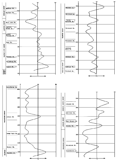
A detailed discussion of the features of Figure 1 will not be undertaken because the connection with reality is at best problematic. However, the following feature of Figure 1 is perhaps sufficiently general to be considered "real":

Levels of G are noticably higher in the Kansas City Group and below as well as in the Admire Group and above. Clearly, the interpretation is that the Moore ideal is more descriptive of the "facts" within the middle Missourian through Virgilian of Kansas than elsewhere in the interval considered.

Two points demand mention in connection with the analysis described above.

First, because the input lithologies were visualized as representing a continuous sequence, freedom of choice as to the starting point (transgressive or regressive) could not be allowed for each subsequence. Rather, the distinct values of G, resulting from different starting points were first accumulated and averaged over the entire interval and then minimized to obtain the final G. Each G, represented a single initial choice of transgression or regression (for the first subsequence). Compared to the procedure for calculating G in a single seven-unit sequence, the distinction here is summarized in the statement that reported values were minimized average G (hereafter called MAG) values over the interval.

Secondly, when ideals with six-unit hemicycles are considered there may he as many as four starting points which will yield distinct G_i rather than two. In such cases, the reported MAG was the minimum of the averaged G_i where i = 1,2 or 1,2,3 or 1,2,3,4 depending on certain characteristics of the ideal under consideration.

Analysis of the complete population of ideals showed that no member had MAG less than that of the Moore ideal. For explaining the composite section of the Kansas rock column on the basis of the least-G criterion, the Moore ideal is the best possible sequence among all symmetric ideals with five- or six-unit hemicycles. No basic significance is claimed for this result because, as has been previously mentioned, the data from the Kansas rock column was pre-synthesized and correspondingly unreal. In addition, bias may well have been introduced by the writer during translation of descriptions into numerical sequences.

Figure 1--Variation of G through the idealized composite section (five-point moving average). A larger version of this figure is available.

Distribution of G in a Sample of Rock Sequences

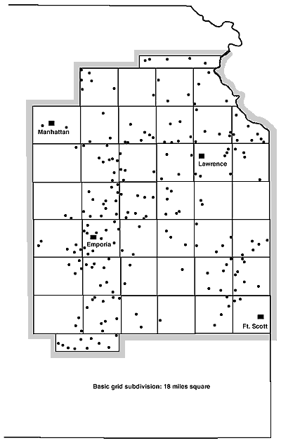
Answers to questions B1, B2, and B3 were obtained from a sample of actual seven-unit rock sequences drawn from available measured sections within the region shown in Figure 2.

The Sample

The State Geological Survey of Kansas kindly made available a file of measured sections and provided a map of locations for an initial selection of about 400 sections. This selection included all available sections which happened to display at least seven lithologic units within the interval from Hepler Sandstone to Roca Shale. The preliminary set of 400 sections was subjected to a sampling procedure as follows:

(1) A grid was superimposed upon the map showing the location of, and stratigraphic group(s) represented in each available section.

(2) The number of available sections per group was tabulated for each grid subdivision.

(3) The total number of sections to be retained was set provisionally at 250, and it was decided that group representation should be proportional to the "size" of the group.

(4) The percent of the total interval actually occupied by each stratigraphic group had been previously estimated by

P_i = (n_i / N) * 100
where p_i = percent of interval represented by the ith group.
n_i = number of recognized lithologies within the ith group, estimated from the Kansas rock column.
N = estimated total number of recognized lithologies in the interval studied.

(5) These considerations dictated that the group representation in the final sample should be as follows:

(6) Where a group was originally represented to excess, sections were discarded from those grid sub-divisions containing the most representatives of the group in question. The particular sections to be discarded were randomly chosen. In this way 250 sections were chosen from the available 400.

(7) Locations of the desired 250 sections were then communicated to Dr. D. F. Merriam, who provided Xerox copies of the measured sections and descriptions. To this point the writer was unaware of the detailed characteristics of the sections to be used.

(8) On each section containing more than seven lithologic units, according to the classification system of Table 2, a starting point was randomly chosen. Upward from this starting point, seven successive units were defined and classified as 1, 2, 3, 4, 5.

(9) For several different reasons, mainly because of difficulty in interpreting descriptions, 15 sections were considered unsuitable and were discarded. The final sample consisted of 235 seven-unit sequences.

(10) To check the percentage of group representation each sequence in the final sample was classified to group. In cases of overlap, the section was counted twice. Compare the break-down below with that of (4).

The chief purpose of this procedure was to insure that the final sample of seven-unit sequences would be spread over the geographic area and the stratigraphic interval of interest. The writer feels that this kind of "representativeness" is a desirable feature of geologic sampling, in which true randomness is usually not at issue. In the present case, certainly, it was not a matter of choosing between the kind of sample obtained and a truly random sample. Ideally, a random sample would have had both locality and stratigraphic interval (group) randomly predetermined. It would have been necessary to be able to go to any locality and there observe a section within any stratigraphic group. The obvious difficulty is that when one is restricted to surface measurements, he is also restricted by the fact that outcrops are where you find them. In addition, it was necessary for this study to consider only those sections already measured and recorded. No sample of the available sections could have been considered a random sample of the population to which inference was to be made, i. e. seven-unit sequences in the three-dimensional area-interval of interest. That the sample actually used was a reasonable approximation to that goal is, at this point, simply assumed.

Figure 2--Distribution of sample localities. A larger version of this figure is available.

A Test for Randomness

The sample was analysed in a manner similar to that already described for the composite section. Differences were as follows:

1. The 235 sections were separate entities and the choice of a minimizing starting point was left open for each seven-unit sequence.
2. The average values of G were determined after the 235 separate minimumizations, hence were average minimum G (AMG) values, rather than MAG values as before.

The G-values corresponding to each observed sequence, with reference to the Moore ideal, formed the basis of a simple test in answer to the question B3. Consider the null hypothesis, H₀:

The sample of observed sequences was drawn from a population described in Table 3, i. e. every conceivable seven-unit sequence had equal opportunity to appear in the sample because the sequences occur randomly in nature.

For the sake of brevity, call this H₀ the randomness hypothesis. The alternative hypothesis, then, is a non randomness or the simple negation of H₀. Table 5 shows the observed number of occurrences for the various G-values, the expected number according to the distribution under H₀ (from Table 3), and calculated quantities necessary for a chi-square test of H₀,where

G = a value of the discordance index.
O_G = the number of times (out of 235) the particular G was observed.
E_G = the number of times the particular G would be expected to have occurred under H₀ (= 235 X column three of Table 3).

Groupings at the extremes of the observed distribution were made in order to satisfy the chi-square requirement that min G (E_G) = 7. The procedure is to calculate the statistic:

and to note that in large samples X² is approximately chi-square distributed under H₀. Reference to tabled chi-square with 13 degrees of freedom (m-1, where m = no. cells used) reveals that under H₀ the probability of observing a X² this large or larger is much less than 0.00001. The randomness hypothesis is most decidely to be rejected. It may be desirable to emphasize the assumptions under which the above chi-square test is a valid rejection of the randomness hypothesis. We assume:

1. That if the recognized lithologies actually occurred in random sequences in nature, then any sequence would be as likely to occur as any other.
2. That the population distribution of G under the randomness hypothesis would be the same as the distribution derived by generating all possible sequences and assigning them equal probabilities.
3. That we have a random sample from the population of interest, namely the population of all seven-unit sequences, within the defined three-dimensional area-interval.
4. That the dependence of the theoretical Gdistribution on the ideal sequence of reference (the Moore ideal) does not affect the test of randomness.

Assumptions (1) and (2) would appear to be justified. Assumption (3) as we have already seen, is invalid but should be approximately true. Assumption (4) is reasonable because the alternative to randomness is unspecific. The particular kind of order we visualize in order to be able to calculate G has no direct bearing on the question, "Does any order exist?". In other words, the test would be expected to reject with any choice of reference sequence.

Table 5--Data for the chi-square answer to B3.

G-values of Alternative Ideals

The AMG values obtained from the analysis of the entire population of 660 distinct ideals will allow no simple interpretation. Of the ideals tested 78 yielded AMG less than that of the Moore ideal. The twenty smallest AMG are listed in Table 6.

Table 6--Value and rank of twenty smallest AMG.

Among this surprisingly large number of "improvements" over the Moore ideal, the best is ...1 2 3 4 5 2 5 4 3.... The chief difference between this and the Moore ideal is the extra unit-2 per hemicycle. Table 7 shows another set of the hemicycles which generate ideals with relatively low AMG. The grouping is intended to illustrate some of the reasons for the results obtained. Note first that all ideals shown have six-unit hemicycles, and the unit repeated in the hemicycle is either 2 or 3. Both of the observations hold for all 78 "improvements."

Table 7--Selected AMG showing relationships: * indicates reverse of a previously listed hemicycle.

Table 8 shows the distribution and frequency of the recognized units among the positions (a₁) of the sample sequences. The high proportions of units 2 and 3 would seem to account for the fact that ideals with extra units 2 or 3 have low AMG, other factors remaining constant. Note also the low proportion of unit-1 in the sample. Table 7 shows that the position unit-1 occupies has relatively little effect on the value of AMG. In the first group of four ideal hemicycles, for instance, the change in position of unit-1 from a₁ to a₄ caused the change in AMG rank from 1 to 7.

Table 8--Distribution and frequency of recognized lithologic units in the sample of seven-unit sequences.

In summary, the relative proportions in the sample of the units 1-5 interact with the ordering of these units in the ideal and AMG is a complex function of both. This should have been obvious at the outset. Are all 78 ideals with low AMG to be considered improvements over the Moore ideal? If the classification of lithologies were entirely objective and unambiguous, the answer would be an unqualified yes.

Problems of Classification

The classification used here is deficient. It has already been mentioned that the tie-breaking "position" criterion begs the question. In a sense, the use of such a criterion is the most serious deficiency of this study. In another sense, it is largely irrelevant. Given criteria adequate to assign every lithology in the chosen area-interval to one of the recognized a priori classes, the need for tie-breaking would have been automatically removed. This study has been chiefly concerned with the mechanical procedures whereby useful conclusions would be reached, given, as a point of departure, just such an objective and unambiguous classification of cyclothemic units.

The following brief discussion is intended as the barest food for thought concerning the difficulties to be encountered in any future attack on problems of classification. The discussion is in terms of the specific questions asked here, but the implications are more general.

Fusulinid Requirement

In the Moore ideal, the type-5 unit is pivotal between the hemicycles in such a way that if physical transgression and regression is visualized, then unit 5 represents maximum transgression or the so-called "deep-water" limestone. It may be true that the presence of fusulinids is one of the best criteria for recognizing such a unit. Still, the type-5 unit which contains fusulinids at one locality may be physically continuous with a limestone which is type-3 at another locality because fusulinids are lacking. If a true facies change is so indicated, such a situation need not concern us too much. On the other hand, if other faunal elements remain the same we may legimately wonder whether presence of fusulinids is that important. With special regard to the present study, it is probable that fusulinids may be lacking in the descriptions of some measured sections though present at the outcrop.

Inclusiveness of Unit 3

The limestones encountered in the sections used for this investigation are fusulinid-bearing, fossiliferous (no fusulinids), or unfossiliferous; massive to thin bedded and often wavy bedded; hard and dense to soft, argillaceous or "punky"; pure to ferruginous or otherwise impure; and so forth. Almost any combination of such adjectives describes some limestone in the interval considered. In what sense can all nonfusulinid limestones be considered equivalent? In particular it seems likely that the many impure and thin-bedded limestones interbedded with shales and not distinguished as members should be separated from other type-3 units.

Inclusiveness of Unit 2

A similar objection can be made concerning the criteria for recognizing unit 2. As a general rule, the shales of the interval considered tend to be less fossiliferous than adjacent limestones. This alone accounts for the scarcity of positively identifiable type-4 units, and the majority of shales became type-2 by default as it were. Unit 2 may be marine or nonmarine, fossiliferous or unfossiliferous, and any color at all.

Degree of Clasticity for Unit 1

An attempt to use the classification of Table 2 on descriptions of measured sections is especially difficult when the terms siltstone, mudstone, and conglomerate are encountered. Is siltstone to be called sandstone or shale? Is mudstone to be considered shale, or, if calcareous, impure limestone? What about conglomeratic limestones? The relative scarcity of type-1 units in the sample is probably "real" regardless of classification difficulties, but we may wonder whether the presence of sandstone is really an environmental measure. The sandstone environment, whatever it may be, could have been present at many points in time which did not happen to coincide with a supply of coarse clastics.

Thickness

Thickness is a criterion whether it should be or not. For this investigation, all lithologic units less than 0.3-feet thick were ignored. Clearly there must be some such arbitrary cut-off point. Is it then reasonable to assign equal weight to all limestones, for instance, from 0.3 to 20 feet in thickness?

Generalizations and Directions

We may distinguish at least three types of troublesome questions stated or implied in the above discussion:

1. How many lithologies should be recognized?
2. What combination of criteria will effect the assignment of actual rock units to the n recognized categories without ambiguity?
3. Given an appropriate set of criteria, how should they be weighed, i.e. what is the order of their relative importance?

There exists no set procedures to tell us which criteria may be of importance, but intuitively we may conclude that it will be necessary to consider many types of criteria. Surely an objective synthesis should draw information from many fields. Paleontology, mineralogy, petrology, sedimentology, geochemistry, all may be called upon to contribute to the store of measurable variables from which a set of criteria appropriate for the purpose at hand may somehow be chosen. A subjective guiding principal for preliminary selection of criteria would include an evaluation, in terms of current geologic thought, of the "amount of information" about ancient environment contained in any particular variable.

Various types of cluster and factor analysis exist which could be applied to such preliminary criterion matrices, and in theory at least, useful answers to questions like (1) and (2) would eventually result. For an interesting example of factor analysis applied to a geologic problem see Imbrie and Purdy (1962). Question (3) could then be approached in a relatively straightforward manner through the use of discriminant functions.

Development of a fully objective classification designed specifically for an investigation such as this would be a long and arduous task. By side-stepping the difficult job and anticipating some of the potential returns on such an investment of effort, this study may serve as some small motivation.

Conclusions

It is easy to see, in restrospect, that the classification used here was such that the preponderance of units 2 and 3 in the sample was inevitable. Any change in the classification which tended to equalize the proportions of the recognized units would probably tend to reduce the number of improvements on the Moore ideal. Of course, this is not to be considered a goal, i. e. justification of the appropriate criteria must be based on independent evidence.

The purpose of this investigation will have been served if any motivation has been provided toward the development of an objective classification based on geochemical and lithologic indicators of environment. In addition it is hoped that the distinction is fully grasped between what is reasonable and what is demonstrable. In the opinion of the writer, there is some degree of evidence here that the Moore ideal cyclothem is, after all, the truth behind the complexity of the observable quantities. But opinion is relatively worthless. Refinement of the criteria for classification may ultimately render the truth susceptible to demonstration by methods similar to those developed here.

In the meantime, geology as a scientific discipline needs more and better attempts to demonstrate the truth of its reasonable hypotheses. If nothing else, such attempts will often demonstrate that our basic methods of observation, measurement, and classification are inadequate to deal systematically with the larger problems. We need to become increasingly aware that the only slightly exaggerated formulation, "How do you feel about cyclothems?", is simply not a scientifically meaningful question. We need to become increasingly willing to focus our attentions on hypotheses at least potentially susceptible to proof and on methods oriented toward the realization of that potential.

References

Imbrie, John, and Purdy, E. G., 1962, Classification of modern Bahamian carbonate sediments, in Classification of carbonate rocks: Am. Assoc. Petroleum Geologists Mem. 1, p. 253-272.

Moore, R. C., 1936, Stratigraphic classification of the Pennsylvanian rocks of Kansas: Kansas Geol Survey Bull 22, 256 p. [available online]

Moore, R. C., and others, 1951, The Kansas rock column: Kansas Geol Survey Bull 89,132 p. [available online]

Pearn, W. C., 1964, Finding the ideal cyclothem: Unpub. master's thesis, Kansas State University, 62 p.

Kansas Geological Survey
Comments to webadmin@kgs.ku.edu
Web version Feb. 2003. Original publication date Dec. 1964.
URL=http://www.kgs.ku.edu/Publications/Bulletins/169/Pearn/index.html