| Original published in W.W. Hambleton, ed., 1959, Symposium on Geophysics in Kansas: Kansas Geological Survey, Bulletin 137, pp. 225-240 | ||
Central Exploration Company, Inc.
The complete article is available as an Acrobat PDF file.
Many of the structures of Kansas are small and of low relief. The unknown quantities assumed in conventional seismic computation may result in errors of such magnitude that they completely mask oil field structures or relative dip adjacent to points of geologic control. Improvement in recording techniques and interpretation has decreased this error greatly. Knowledge, gained only by experience with many problems, makes the seismologist aware of the cause of error. This paper lists many of the problems and suggests new methods of solving them.
The seismograph has been a very important and valuable tool for oil exploration in Kansas throughout the years. It has been successful; it is relatively inexpensive and, combined with shallow subsurface information obtained from electric logs, is becoming more and more accurate.
Although seismic record quality in Kansas generally is good, many of the oil field structures are of such low relief that they can be discerned only through close approach to the normal limits of seismic accuracy. The major seismic problems are found in shallow formations, from the surface down to the Stone Corral anhydrite of Permian age. Lesser problems are caused by deeper formations. Concentrated study and research by the geologist and geophysicist on the shallow formations is necessary in locating the new oil fields, which are increasingly more difficult to find.
This paper lists briefly the problems that arise in interpreting seismic data in Kansas and suggests possible methods for overcoming some of these difficulties.
Unusual conditions in Kansas introduce errors in conventional seismic methods of computation. Some of the problems facing the interpreter of seismic data are discussed below. The weathering problem is omitted because it is universal.
Areas of irregular topography in some parts of Kansas are characterized by greater average velocities on hills, as compared with average velocities in valleys. It has been suggested that the additional sediment weight causes higher velocities. Insufficient research has been conducted in Kansas to prove this conclusion or to establish a usable velocity ratio for hills and valleys.
Different kinds of outcropping rocks in the same area are a source of near-surface velocity variation. In addition, record quality is poor, owing to "character" changes and "phasing." In such areas, field procedure usually is altered so that explosive charges are placed in geologically comparable material. This methods of correction requires much experimentation in the field. Parts of Rooks and Ellis counties are typical problem areas.
Inasmuch as Pleistocene or Tertiary mantle rock has a low velocity, it must be treated as a second weathering layer, which must be penetrated by the shot hole or measured for velocity. This mantle rock is as much as 750 feet thick and in places has a very irregular bedrock contact. If shot-hole penetration is not economically feasible, interval maps are used.
In Kansas, a regional southward velocity increase is found in rocks below the Stone Corral anhydrite. The problem is especially vexing where there is insufficient velocity control.
The salt of the Wellington formation of Permian age has a much higher seismic velocity than the overlying or underlying shales. Problems arise because of, thickness and velocity changes from one shot hole to the next. The velocity changes are caused by variation in salt density. In such areas conventional seismic maps are in error on horizons below the salt; time-isopachous or "isotime" maps using the Stone Corral anhydrite as a datum also are in error. Data on deeper beds are obtained from interval maps based on two reflections below the salt; it is assumed that thinning is the result of structure. Record quality must be at its best for precise construction of interval maps.
The Blaine salt, a salt of the Blaine formation, causes error also because of thickness and velocity change, but because the salt is relatively shallow, "isotime" maps usually are accurate. Widess (1952) has discussed the seismic problems due to the Blaine salt in the Blaine Salt Basin for an area in and adjacent to Clark County, Kansas.
The "isotime" method of seismic interpretation (discussed more fully under Method of Interpretation) is based on the assumption that the reference plane is flat. The assumption may not be valid. For example, the Stone Corral anhydrite, a widely used reference marker, is not flat in many areas and the irregularity causes errors in interpretation.
The rocks of Kansas are sufficiently conformable that most seismic reflections are of adequate quality, even though velocity control for depth computation and identification of mappable stratigraphic horizons is sparse. One notable exception is the erosion surface at the top of the Arbuckle, which may yield no reflection or one too complex to be discerned on the records. The low areas of this old Arbuckle surface usually are filled or partly filled with conglomerate. It is possible that detailed velocity studies of conglomerate and Arbuckle may reveal a velocity difference of sufficient magnitude that the Arbuckle lows can be determined by measuring time differences from a Lower Pennsylvanian reflection to a reflection within the Arbuckle.
Many of the problems of seismic interpretation cannot be solved by any single method of interpretation. Indeed, it is likely that experience and good velocity control are the most important factors in successful interpretation. Figure 1 shows the location of some typical seismic records (Fig. 2, 3, 4, 5) in various Kansas counties, which may aid the geophysicist in acquiring familiarity with Kansas records and record quality. An aid to velocity control is the partial list (Table 1) of well velocity surveys in Kansas through 1957. This list was taken mainly from the compilations of wells shot for velocity (Swan, 1944, 1946, 1949, 1951; Gaither, 1956, 1957,1957a).
Figure 1--Map showing location of seismic records.
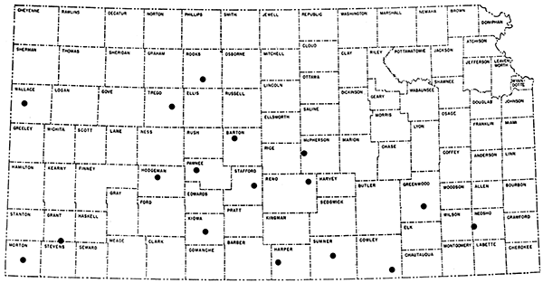
Figure 2--Typical seismic records, Kansas counties.
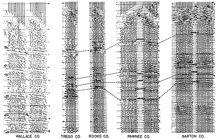
Figure 3--Typical seismic records, Kansas counties.
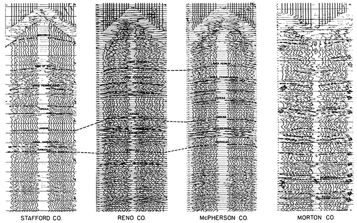
Figure 4--Typical seismic records, Kansas counties.
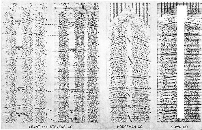
Figure 5--Typical seismic records, Kansas counties.
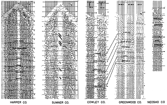
Table 1--List of wells shot for velocity in Kansas through 1957. [Gaither 1956, 1957, 1957a; Swan 1944, 1946, 1949, 1951; by permission of Society of Exploration Geophysicists and others. Abbrevations: CSO, Cities Service Oil Co.; GGC, General Geophysical Co.; GRC, Geophysical Research Corp.; GSI, eophysical Service, Inc.; KVI, Key Velocities, Inc.; OKSWA, Oklahoma-Kansas Well Shooting Association; SGC, Southern Geophysical Co.; SSC, Seismograph Service Corporation; WGC, Western Geophysical Co.]
| County | Company | Lease | Location | Survey depth |
Shot by | Date | Sponsored by |
|---|---|---|---|---|---|---|---|
| Barber | Drillers Gas | No. 2 Skinner | 9-31S-14W | 4,325 | KVI | 1946 | KVI |
| Barber | Champlin Ref. Co. | Beardmores Calloway | 20-31S-12W | 4,663 | Champlin | ||
| Barber | Continental | No. 1 Lake | SE SE SW 11-32S-14W | 4,918 | KVI | 1946 | KVI |
| Barber | Pure | No. 1 Palmer | SE NE SW 10-33S-10W | 4,700 | SSC | 1937 | OKWSA |
| Barber | Lindas & Armer, et al. | No. 1 Pfaff | NW SE NE 15-34S-10W | 5,301 | KVI | 1948 | Atlantic |
| Barber | Barber Oil Co. | No. 1 Brach | 17-34S-15W | 5,549 | National | 1954 | Chicago Corp. |
| Barber | Chicago Corp. | Barabara Oil No. 1 Brach | 17-34S-15W | 5,549 | Champlin | ||
| Barber | Conoco and City Prod. | No. 1 Sternberger | 5-35S-13W | 5,584 | Conoco | 1955 | OKWSA |
| Barton | Sinclair-Pro | No. 1A Davidson | 9-16S-11W | 3,343 | Petty | 1937 | OKWSA |
| Barton | C. C. Millerd Sy | No. 1 Boertz | 13-18S-12W | 3,400 | GRC | 1931 | |
| Barton | Derby Oil | No. 1 Berscheidt | 12-20S-11W | 3,000 | GRC | 1932 | |
| Barton | Atlantic | No. 1 Schneider | 15-20S-13W | 2,438 | 1933 | ||
| Brown | Carter | No. 1 Strat. Test | SW SW SW 24-4S-16E | 3,475 | Carter | 1939 | |
| Chautauqua | Frankfort | No. 1 Brazle | 11-33S-9E | 2,750 | SSC | 1955 | Frankfort |
| Clark | Olson Oil | No. 1A Morrison | C SE SW 17-32S-21W | 6,458 | GSI | 1941 | |
| Comanche | Conoco | No. 1 Cole | 8-34S-18W | 6,426 | Mayes-Bevan | 1955 | Conoco-Pure |
| Comanche | Pure | No. 1 Beal | 5-34S-17W | 5,937 | SSC | 1955 | Conoco-Pure |
| Cowley | Barrett, et al. | No. 8 Waite | SW NW 21-31S-4E | 3,100 | Shell | 1939 | OKWSA |
| Cowley | Carter | No. 1 Radcliff | 32-32S-7E | 2,780 | Carter | 1951 | Carter |
| Cowley | Texas | No. 1 Walton | 31-33S-4E | 3,724 | SSC | 1956 | Texas |
| Decatur | Helmerich-Payne | No. 1 Penn | NW NW SW 16-2S-29W | SSC | 1943 | Texas | |
| Decatur | Stanolind | No. 1 Hale | SE SE SE 32-2S-26W | 4,019 | Stanolind | 1943 | |
| Edwards | Kewanee | No. 1 Samuel | 29-24S-19W | 5,053 | SSC | 1956 | Kewanee |
| Edwards | Stanolind | No. 1 Arensman | NE SE 23-25S-19W | 5,065 | Stanolind | 1941 | OKWSA |
| Edwards | Amerada | No. 1 Tansil | 32-25S-19W | 4,950 | GRC | 1929 | |
| Ellis | Stanolind | No. 1 Furthmeyer | SE SE SE 25-12S-16W | 3,025 | GSI | 1932 | OKWSA? |
| Ellis | Darby | No. 1 Younger | NW NW NW 20-13S-17W | 3,605 | SSC | 1941 | Sunray? |
| Ellis | Pam Kar | No. 1 Moore | 32-14S-19W | 3,743 | Westem | 1955 | Stanolind |
| Ellsworth | Frankfort | No. 1 Kuch | 8-14S-10W | 4,290 | SSC | 1955 | Frankfort |
| Ellsworth | Gypsy | No. 2 Kozisek | NE SE SE 16-16S-10W | 3,300 | SSC | 1934 | OKWSA |
| Finney | Shell | No. 1 Case | NE SE NW 7-21S-30W | 5,530 | SGC | 1950 | Shell |
| Finney | W. L. Hartman | No. 11 Damme | 21-22S-33W | 4,676 | Central | 1953 | W. L. Hartman |
| Finney | Conoco | No. 1 Kleysteuber | 29-26S-31W | 5,662 | Conoco | 1953 | Conoco |
| Graham | Shell | No. 8 Knipp | SE SW 14-9S-21W | 3,835 | Shell | 1948 | Shell |
| Gray | Champlin | No. 1 Becker | C NE SW 34-28S-29W | 6,270 | Stanolind | 1939 | OKWSA |
| Hamilton | Barnsdall-Denv. | No. 1 Porter | SW NE 30-25S-41W | 3,000 | Shell | 1937 | OKWSA |
| Hamilton | Shell | No. 1 Scott | SW NE 28-22S-43W | 5,525 | KVI | 1948 | KVI |
| Harper | Barry | No. 1 Anthony | 17-31S-9W | 4,812 | GRC | 1934 | GRC |
| Harper | Texaco | No. 1 Baker | 24-34S-5W | 5,091 | Texaco | 1952 | Texaco |
| Harper | Texaco | No. 1 Harrison | 13-33S-6W | 5,026 | Texaco | 1955 | Texaco |
| Harper | Gulf | No. 1 Rife | 31-33S-6W | 5,133 | Conoco | 1954 | Conoco |
| Harper | Anschutz | No. 1 Hoyt | 7-33S-8W | 5,075 | Conoco | 1955 | Conoco |
| Harper | Texaco | No. 1 Baker | 24-34S-5W | 5,091 | Texaco | 1952 | Texaco |
| Harper | Amerada | Mandeville | 24-34S-6W | 4,761 | GRC | 1929 | GRC |
| Harper | Amerada-Dixie | No. 1 Misak | 25-34S-6W | 5,100 | GRC | 1931 | |
| Harvey | Shell | No. 1 Neufeldt | SE SW NW 8-22S-3W | 3,406 | SSC | 1934 | OKWSA |
| Haskell | Huber and Conoco | No. 1 Weirauch | 23-28S-31W | 6,480 | GGC | 1955 | Conoco |
| Hodgeman | Shell | No. 1 Springer | SE SW SW 24-22S-24W | 5,100 | SGC | 1950 | Shell |
| Hodgeman | Armer-Koplin | No. 4 Schraeder | SE NW NW 3-24S-24W | 5,223 | National | 1951 | Armer-Koplin |
| Keamy | Stanolind | No. 1 Judd | SE SE 15-21S-38W | 5,275 | Stanolind | 1940 | Stanolind |
| Kingman | Jack Heathman | No. 1 Woodridge | 16-27S-7W | 4,301 | Central | 1954 | Heathman |
| Kingman | Skelly | No. 1 Rouse | C N/2 SE 20-27S-10W | 4,282 | Empire | 1934 | OKWSA |
| Kingman | Texaco | No. 1 Callison | 31-29S-5W | 4,561 | Texaco | 1954 | Texaco |
| Lane | Virginia Drlg. Co. | No. 1 Harper | 26-16S-30W | 5,200 | SSC | 1957 | Phillips |
| Logan | Gruenerwald | No. 1 Swart | 12-11S-32W | 4,757 | Central | 1956 | OKWSA |
| Logan | Texas | No. 1 Smith | NE NE SW 30-11S-36W | 5,321 | Texaco | 1943 | OKWSA |
| Logan | Wycoff Bros. | No. 1 Uhland | 8-14S-35W | 4,888 | SSC | 1956 | Phillips |
| Lyon | Wilkinson Drlng. Co. | No. 1 Gregory | 30-15S-10E | 3,301 | SSC | 1957 | Carter |
| McPherson | Darby | No.5 Coons | NW NE SW 20-19S-1W | 3,361 | SSC | 1934 | Carter |
| Meade | Texaco | No. 1 McJones | 19-33S-29W | 5,870 | Texaco | 1956 | Texaco |
| Meade | Helmerich-Payne | No. 1 R. E. Adams | SW NW 11-35S-29W | 6,150 | Gulf | 1946 | OKWSA |
| Mitchell | Carter | No. 1 Victor (Strat. Test) | SE SW 20-9S-7W | 3,725 | Carter | 1939 | |
| Morris | Stanolind | No. 1 B. V. Carpenter | 29-17S-7E | 2,148 | Central | 1955 | Stanolind |
| Morris | Fred Drolte | No. 1 T. Loy | 28-17S-9E | 3,224 | SSC | 1956 | Carter |
| Morton | Colorado Oil & Gas | No. 1 Hayward | 9-32S-42W | 5,218 | Central | 1952 | Colorado Oil & Gas |
| Nemaha | Carter | No. 1 Gillbert Land Bank | NW NW SE 14-2S-14E | 3,228 | Carter | 1949 | Carter |
| Ness | Atlantic | No. 1 J. R. Elmore | 7-16S-21W | 4,472 | Central | 1955 | Atlantic |
| Ness | Gulf | No. 1 Keough | 3-18S-21W | 4,600 | SSC | 1956 | OKWSA (Conoco) |
| Osborne | Carter | No. 1 Neushwanger | SW NE SW 15-8S-14W | 3,774 | Carter | 1943 | Carter |
| Osborne | N. Ordnance | No. 1 Vandement | C NW NW 3-9S-13W | 4,118 | Carter | 1943 | Carter |
| Ottawa | Stanolind | No. 1 Duggan | NW NW SW 12-12S-1W | 3,360 | Stanolind | 1943 | |
| Pawnee | Bennett & Roberts | No. 1 Fox | 31-21S-18W | 4,517 | SSC | 1956 | Conoco |
| Pawnee | Adair & Morton | No. 1 Thompson | NW NE NW 16-22S-20W | 4,960 | SSC | 1942 | OKWSA |
| Phillips | Carter | No. 1 Robb | SE SW 3-4S-18W | 3,574 | Carter | 1942 | Carter |
| Pratt | Skelly | No. 1 Gilcreast | C SE 7-28S-11W | 4,200 | SSC | 1935 | OKWSA |
| Pratt | Lion | No. 1 Mico | 30-29S-11W | 5,164 | Tomlinson Geo. | 1956 | Lion |
| Pratt | Lario | No. 1 Lemon | SE SE NW 12-29S-13W | 4,360 | GRC | 1936 | OKWSA |
| Reno | Roth & Faurot | No. 1A Yoder | C NW NW 15-24S-5W | 3,915 | SSC | 1934 | OKWSA |
| Reno | T & M Oil and Tom Allen | No. 1 Stewart | 16-24S-6W | 4,171 | Tomlinson Geo. | 1956 | Lion |
| Reno | Tatlock Oil | No. 1 Vernon Tonn | 17-25S-4W | 4,000 | GRC | 1932 | |
| Reno | Stanolind | No. 1 Hilger | SE SE NW 16-26S-4W | 3,944 | GRC | 1936 | OKWSA |
| Reno | Sinclair-Pro | No. 1 Shephard | SE SE NW 22-26S-9W | 4,333 | SSC | 1934 | OKWSA |
| Rice | Continental | No. 1A Lansing | NE NE SW 25-18S-SW | 3,100 | GRC | 1934 | OKWSA |
| Rice | Elwell, et al. | No. 1 Springer | NW NE NW 35-18S-10W | 3,273 | SSC | 1934 | OKWSA |
| Rice | Nickerson, et al. | No. 1 Lyons | SE NW 27-20S-SW | 3,559 | Petty | 1935 | OKWSA |
| Rice | Cities Service | No. 1 Heckel | NW NW SW 18-20S-9W | 3,303 | CSO | 1934 | CSO |
| Rice | Deitrick, et al. | No. 1 Fitzpatrick | C NE NE 30-21S-SW | 3,628 | SSC | 1934 | OKWSA |
| Rush | Republic Nat. | No. 1 Eva Webb "C" | 16-19S-20W | 4,200 | SSC | 1954 | Republic |
| Rush | Conoco | Solar No. 1 Schmidt | 2S-16S-19W | 3,840 | SSC | 1956 | Conoco |
| Russell | Empire | No. 1 Ehrlich | NE NE SE 2S-13S-14W | 3,274 | GRC | 1935 | OKWSA |
| Russell | ElDorado | No. 1 Strattman | SW SE SE 32-14S-11W | 3,210 | SSC | 1934 | OKWSA |
| Russell | Empire | No. 1 Mai | C NW SW 24-15S-14W | 3,247 | SSC | 1934 | OKWSA |
| Scott | Atlantic | No. 1 Dague | C SW NW 14-20S-33W | 4,563 | WGC | 1935 | OKWSA |
| Sedgwick | Empire | No. 1 Shawver | NE NE NE 13-28S-2W | 3,704 | GRC | 1934 | OKWSA |
| Sedgwick | O. A. Sutton | No. 1 Peltz | SE SE NW 32-2SS-2W | 4,202 | Central | 1954 | O.A. Sutton |
| Sheridan | Continental | No. 1 Pope | SW SW SE 18-7S-29W | 4,779 | SSC | 1950 | Conoco |
| Sherman | Kingwood-Aurora | No. 1 Rauckman | 11-8S-40W | 5,565 | National | 1952 | Kingwood |
| Sherman | Sinclair-Pro | No. 1 Mercer | NE NW 28-10S-40W | 5,686 | SSC | 1942 | OKWSA |
| Stafford | Shell | No. 1 Schilling | C SW NW 26-21S-13W | 3,721 | SSC | 1934 | OKWSA |
| Stafford | Trigg & Allen | No. 1 Helmers | 2-22S-12W | 3,600 | GSI | 1940 | |
| Stafford | Midwest Refg. | No. 1 Richardson | 36-22S-12W | 3,509 | GSI | 1932 | |
| Stafford | Atlantic | No. 1 Hohner | SE NE 31-23S-14W | 4,077 | SSC | 1935 | |
| Stafford | Shaffer | No. 1 Newell | NE SE 20-24S-11W | 4,050 | Stanolind | 1938 | |
| Stafford | Stanolind | No. 1 Ray McComb | NE NE 27-24S-11W | 3,850 | Stanolind | 1938 | |
| Stafford | Rose Spring | No. 1 Toland | NW NW SE 2-25S-14W | 3,000 | SSC | 1935 | OKWSA |
| Stanton | Killman & Hurd | Rorick Unit No. 1 | 18-30S-42W | 5,460 | SSC | 1956 | Superior |
| Sumner | Carter | No. 1 Weber | C NW SE 26-31S-4W | 4,617 | Carter | 1945 | Carter |
| Sumner | Wentz-Conoco | No. 1 Kern | SE SE NE 6-34S-2W | 4,500 | GSI | 1934 | OKWSA |
| Sumner | Texas Co. | No. 1 Hobbisiefkin | 3-35S-3W | Texaco | 1950 | Texaco | |
| Thomas | Texas | No. 1 Daugherty | NW SW SW 23-6S-33W | 5,023 | Texaco | 1943 | OKWSA |
| Thomas | National Coop. Ref. | No. 1 Wright | 34-7S-36W | 5,040 | SSC | 1956 | Phillips |
| Thomas | Virginia Drlg. Co. | No. 1 Cooper | 12-7S-33W | 4,675 | SSC | 1956 | Phillips |
| Trego | Stanolind | No. 1 F. B. Rinker | SE NE NW 6-12S-22W | 4,171 | WGC | 1954 | Stanolind |
| Trego | Central Comm. | No. 1A Wagg | NW SE 17-13S-21W | 4,494 | SSC | 1936 | SSC |
| Trego | Bennett & Roberts | No. 1 Kline | 19-14S-24W | 4,504 | SSC | 1956 | Conoco |
| Wabaunsee | Carter | No. 1 Dorgan | SW SW NE 6-15S-10E | 3,307 | SSC | 1949 | Carter |
| Wallace | Van-Grisso Oil Co. | No. 1 Frazier Farms | 15-15S-39W | 5,130 | SSC | 1956 | Phillips |
| Wichita | Benedum-Trees | No. 1 Knobbe | 18-18S-35W | 5,101 | SSC | 1957 | Phillips |
In the following paragraphs, the methods of interpretation employed in Kansas are listed with a discussion of the advantages and disadvantages of each and the limit of error involved.
This method of determining thickness of the weathered layer from uphole time is the universal method of seismic computation. Inasmuch as it is familiar to all seismologists, it will be mentioned only brieflly.
Its limitations stem from difficulties in controlling error and from assumptions made in extending of the "weathering" thickness or near surface velocities. It is assumed that the "weathering" at the timing geophones is the same as at the shot hole. The accumulation of slight errors in reading all the various times from the records is another source of error. These errors add up to about .005 second, the usual limit of error acceptable for seismograph work.
This method determines the "weathering" time or depth at the position of the center traces used for timing. When the timing geophones are 55 to 75 feet from the shot hole, the greatest accuracy is obtained and the error can be reduced to about .003 to .004 second.
About .0005 second greater accuracy can be gained by firing the shot so that it explodes at exactly zero time on the record (exactly on a heavy timing line). This is, then, one time that is always zero and no reading error can be made in interpolating the time of the explosion.
The above methods of computation are, of course, also subject to error introduced by velocity changes in rocks between the depth of the shot and the reflecting bed. By drilling 20 to 50 feet into "bed rock," errors caused by the weathered zone at the surface usually can be eliminated. The velocity change from the base of the shot to the Stone Corral anhydrite, possibly the greatest local source of error, is at least partly due to the unconformity between Cretaceous and Permian beds. Most of the regional southward velocity increase in Kansas occurs in rocks below the Stone Corral anhydrite, but seemingly the increase is gradual.
This method has the limitations of the normal uphole and "modified" uphole methods except that it takes into account the regional velocity change. When actual velocities are not available, the map must be constructed by the use of "mis-ties" to wells and its accuracy is dependent on the accuracy of the well tops and the amount of well control. Extreme caution must be used to be certain that the error is not due to miscorrelation. This methods does not appreciably affect definition of local structure and normally is not used, as long as the problem of regional velocity change is considered in the evaluation.
Areas of irregular topography may pose extreme problems in Kansas. It is not unusual to have 200 feet of relief. This method assumes that the average velocity should be applied from the base of the shot rather than adjusted to a flat plane as is in the previously mentioned methods. The "rough topography" method tends to reduce the effect of the topographic changes. It suffers from most of the previously mentioned errors and is used mainly as a check against other methods of computation.
A certain amount of success has been obtained by drilling to a constant datum plane, either into the same formation on all holes or to a level datum plane. Velocity data so acquired have contributed to closer correlation of geologic and seismic information.
In this method, time intervals are determined between reflections from the Stone Corral anhydrite, of Permian age, and reflections from lower rocks of Pennsylvanian, Mississippian, or Ordovician age. The "isotime" method is useful because the accuracy required in many areas of Kansas is much greater than ordinary seismograph methods will allow. The method assumes that the Stone Corral anhydrite is flat or essentially flat and that thinning is due to the structural attitude of deeper beds. It cancels all weathering and velocity errors from the Stone Corral to the surface. Its accuracy is dependent upon the validity of the assumptions, the ability of the interpreter to discern and choose the best data on the recordings and to read record times accurately on the reflections involved, and good record quality. This method has been successful on local structures, but when used on large prospects, the interpreter must keep in mind that in certain areas the anhydrite dips regionally north whereas the lower beds dip regionally south to southwest. The combined dips produce exceptional regional thinning to the north. Here again, most local anomalies are not affected.
The discussion of the previous paragraph indicates that the dip of the Stone Corral is important in mapping areas of large size. The variable-reference-plane method requires construction of a structural contour map of the Stone Corral anhydrite from electric-log and core-drill data. It is not out of order to let the conventional seismic map on the anhydrite influence the contouring of the structural map to a very slight degree.
Time intervals from the anhydrite to the lower reflecting beds are then mapped. These intervals are converted to thickness and applied directly to the sloping anhydrite plane. Maps so constructed tend to be slightly conservative because most real, positive anomalies show to some degree in the anhydrite.
The accuracy of such a method is dependent mainly on the validity of the assumptions regarding the slope of the Stone Corral; the greater the geologic control on the anhydrite, the greater the accuracy. The fact that more and more electric logs are run up through the anhydrite and to the surface is a tremendous aid to the seismologist in Kansas. Anhydrite data used on the shot points are interpolated from the contoured map. A perfect "setup" for this type of computation is in the area of the Hugoton Gas Field of southwestern Kansas, where Permian geologic data are available on one-mile control.
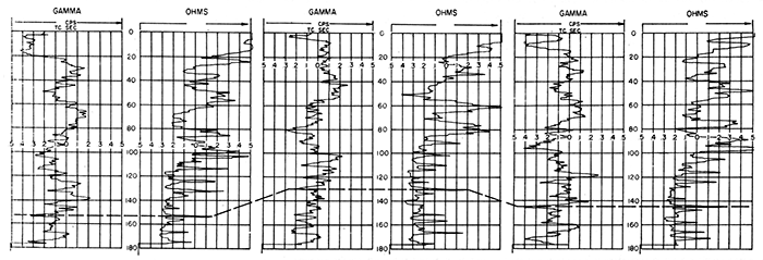
The variablereference-plane method described for the Stone Corral is used, except that more dense control is obtained on shallow horizons. The ideal situation, of course, would be a Stone Corral electriclog datum at every shot point. The cost of obtaining such information would be excessive, but shallow marker beds are almost as useful. It has been discovered that excellent electric-log correlations can be obtained for most of the Cretaceous and Permian sections (Fig. 6). These correlations are surprisingly consistent. Field procedure requires drilling shot holes deeper than usual into bed rock. The cost is not prohibitive and the method attempts to make seismic data in Kansas as accurate as possible.
Figure 6--Electric-radioactivity logs of shot holes in Sumner County showing a shallow Permian marker bed.
The data are computed as above, except that the variable plane is taken from the known electric-log markers on each shot point and the assumption is made that the marker parallels the shallowest consistent reflections. In most areas this reflection surface is the Stone Corral anhydrite, but in some areas, such as parts of Sheridan and Gove counties, it actually is a Cretaceous reflection. In areas where these markers are reasonably near parallel, seismic accuracy has reached a fine point.
There are other areas in Kansas where it is known that the Cretaceous and the Stone Corral markers are not parallel. In many of these areas, the lack of conformity seemingly is manifest by uniform thinning in a definite direction. The amount and direction of thinning can be determined from Stone Corral electric-log information at key wells in the area and shallow log information on the Cretaceous beds at these key wells. By obtaining shallow log or core-drill information over the intermediate area and applying the estimated thickness as determined above, one can make a reliable map on the Stone Corral. Then, by use of time intervals from the Stone Corral to the deeper beds, maps can be made on the Pennsylvanian, Mississippian, and Ordovician beds with a reasonable degree of accuracy.
Other variable reference planes.-The above discussion has been concerned with the area where Cretaceous rocks crop out or lie below the Tertiary and Pleistocene mantle in north-central Kansas. The same method may be applied to the southern and
eastern parts of the state, where Permian and Pennsylvanian beds crop out. Because there is more conformity within the Permian and Upper Pennsylvanian section, the method should be accurate where Permian core markers are applied to lower Permian or upper Pennsylvanian reflections. The time interval from these shallow reflections to lower Pennsylvanian, Mississippian, and Ordovician reflections gives accurate control on these lower beds in most places.
Oil is becoming increasingly difficult to find in Kansas, but more information is becoming available. The fact that more electric logs are run to the surface has been a great aid to the seismologist who is searching for structures in Kansas. All velocity surveys should be conducted to measure the velocity in the Wellington salt. Information can be acquired from study of the Stone Corral anhydrite and the Wellington salt sections of the Permian, and the entire Cretaceous section. It is believed that Permian, Cretaceous, and near-surface rocks create most of the errors and problems of seismic interpretation in Kansas. A thorough study of the attitude, composition, and velocity of the shallow formations is necessary to further improve seismograph accuracy in Kansas.
The seismologist must admit his need for, and accept the advice, suggestions, and cooperation of the geologist in solving the problems of oil exploration.
Gaither, V. U. (1956) Index of wells shot for velocity (fourth supplement): Geophysics, v. 21, no. 1, p. 156-178.
Gaither, V. U. (1957) Index of wells shot for velocity (fifth supplement): Geophysics, v. 22, no. 1, p. 120-135.
Gaither, V. U. (1957a) Index of wells shot for velocity (sixth supplement): Geophysics, v. 22, no. 5, p. 60-79.
Swan, B. G. (1944) Index of wells shot for velocity: Geophysics, v. 9, p. 540-559.
Swan, B. G. (1946) Index of wells shot for velocity: Geophysics, v. 11, p. 538-546.
Swan, B. G. (1949) Index of wells shot for velocity (second supplement): Geophysics, v. 14, p. 58-66.
Swan, B. G. (1951) Index of wells shot for velocity (third supplement): Geophysics, v. 16, p. 140-152.
Widess, M. B. (1952) Salt solution, a seismic velocity problem in western Anadarko basin, Kansas-Oklahoma-Texas: Geophysics, v. 17, no. 3, p. 481-504.
Kansas Geological Survey
Comments to webadmin@kgs.ku.edu
Web version Dec. 6, 2013. Original publication date 1959.
URL=http://www.kgs.ku.edu/Publications/Bulletins/137/Glover/index.html