Kansas Geological Survey, Open-file Report 2004-66
by
Saibal Bhattacharya, Martin K. Dubois, and Alan P. Byrnes
Kansas Geological Survey, Lawrence, Kansas
KGS Open File Report 2004-66
This study pertains to the geologic modeling of sections within the Hugoton-Panoma gas field, and then using reservoir simulation to validate the underlying geologic models. It is hoped that such detailed characterization studies will enable better understanding of these complex and huge gas reservoirs so that plans can be set afoot to economically exploit their remaining potential. The studies and experiments described in this report characterize the Chase and the Council Grove (CG) reservoirs at a variety of scales--single and multiple wells. Initial studies focused on single well, data-rich areas to understand reservoir dynamics, issues related to upscaling and fluid flow, and validate lithofacies based petrophysical relationships developed from available core plug data. Modeling and simulation of the Alexander D unit is the initial step of larger modeling and simulation exercises planned as part of the Hugoton Asset Management Project (HAMP, http://www.kgs.ku.edu/HAMP/index.html).
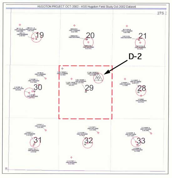
The Alexander D unit (Figure 1A), Section 29, Township 27 South, Range 35 West, Grant County, Kansas, is a one-square-mile producing gas unit in the Hugoton and Panoma Fields in southwest, Kansas. Two wells produce from the Chase Group (Hugoton Field) and a third produces from the Council Grove Group (Panoma Field), both Permian age. Though the Chase (Hugoton) directly overlies the Council Grove (Panoma), the two fields are regulated as separate fields. Three stages of development were the initial Hugoton well, the Alexander D-1 well Hugoton "parent"), followed by the Alexander D-2, the Panoma well, and finally the Alexander D-3, a Hugoton infill well. In this exercise we first modeled and simulated the Alexander D-2 as if it were completed in a separate reservoir, the Council Grove Group. In a later study (KGS OFR 2004-67), we modeled and simulated the Chase and Council Grove reservoirs as if they were one connected system.
Figure 1a--Location of Alexander D-2 well compared to surrounding wells.
The principal properties required for reservoir simulation studies are porosity, permeability, and Sw. However, since Sw cannot be accurately estimated from wireline logs due to deep filtrate invasion during drilling, Sw must be estimated based on lithofacies-dependent capillary pressure relationships (Dubois and others, 2003). Thus, projecting lithofacies in the 3D model space is a critical first step. For these exercises we have assumed that the layered flow units of both the Council Grove and Chase are laterally continuous across the entire unit and that the lithofacies within these units have the same degree of continuity. Properties in the model vary between layers but not within layers. This assumption is based upon the general observation that the lateral scale of major lithofacies bodies is much greater than the scale of the production unit being modeled.
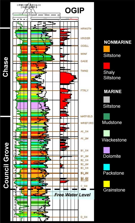
The main flow units are relatively thin (2-10 meter) marine carbonates that are separated by thin (2-10 meter) nonmarine siltstones that have low permeability. The alternating layers were deposited as a series of stacked marine-nonmarine sedimentary cycles (Figure 1B). For the Council Grove (Panoma model) the 233-foot thick interval was divided into one-foot layers and lithofacies were assigned from examination of actual core. Porosity at a one-foot scale was derived from wireline logs and was corrected based upon empirical relationships developed on core data. Permeability and water saturations were estimated at the one-foot scale given porosity and lithofacies using core-derived empirical relationships. Figure 1B shows the stratigraphic section for the Chase and Council Grove Groups with wireline log curves. Color fill are lithofacies. Original gas in place (OGIP) is property-based volumetric for a free water level = 55 feet above sea level and bottomhole pressure = 465 psi.
Figure 1b--Wireline log for Alexander D-2 annotated with lithofacies and original gas in place values.
The Panoma (Council Grove) 3D cellular model was constructed in Petrel, a Schlumberger modeling application, initially having 14,912 cells (233 layers and 64 cells per layer). The cell dimensions (XYZ) were 660 feet X 660 feet X 1 feet and cells were populated with porosity, horizontal permeability, and water saturations by layer. The 14, 912 cell fine scale model was exported from Petrel for simulation and the ASCII file was modified to accomodate a one-foot wide vertical hydraulic fracture.
Alexander D2 well (hence forth called the D2 well) is located (Figure 1A) in Section 29 (27S-35W) in Grant County, Kansas, and was drilled in July 1975 to produce from the CG. This well has produced about 1.6 bcf to date. A continuous core was available for study at this well. Detailed characterization studies were carried out on this core, with facies identification and measurement of porosity and permeability at half-foot intervals. Based on the depositional environment of the CG reservoirs and the data available from the core, a 3D reservoir geomodel was constructed for the drainage area around this well. Based on the petrophysical data measured on plugs taken from this and other wells in the study area, facies-based capillary pressure (Pc) equations were developed. Log derived water saturations (Sw) values are unreliable in Hugoton field due to invasion problems. Thus, facies-based Pc equations were used to estimate initial Sw given a FWL--determined from production and DST data.
Figure 2 shows the porosity, permeability, and initial Sw distribution at the D2 well on a one-foot scale. For purposes of fine-scale reservoir simulation, adjacent one-foot water saturated intervals (Sw = 1) were upscaled into one layer. Thus, layer 1 extends from 2886 feet to 2889 feet while each one-foot interval where Sw was less than 1.0 was named as a separate individual layer. Figure 3 shows that following the above process, the initial fine-scale reservoir model for the D2 well consisted of 96 layers. Figure 4 summarizes the major elements included in the simulation model for this well. In the Hugoton and Panoma fields, most wells (including D2) were fractured during completion. Based on shut-in test data from D2, the fracture half length was estimated to be between 210 feet to 337 feet based on assumed fracture heights ranging from 211 feet to 83 feet. D2 is one of the most productive wells in its neighborhood, and thus a fracture length of 660 feet was assumed in this study.
Figure 2--Numbering of Layers--Fine scale model. Calculated OGIP = 1,906,490 MCF.
| Perfs recorded: Scout Card | |
| 2890 | 2902 |
| 2944 | 2950 |
| 2954 | 2966 |
| 2976 | 2984 |
| 2992 | 3016 |
| Depth | Arithmetic average | Rel K Number |
HFW | SW | MCF per acre-ft |
MCF per section |
Zone | Associated OGIP |
Perf | Simulation Layer |
|
|---|---|---|---|---|---|---|---|---|---|---|---|
| Upscale Phi_Corr |
In-situ Permeability |
||||||||||
| 2886 | 0.0780 | 0.002658 | 1 | 194 | 1.000 | 0.0 | 0 | A1_SH | 88,109 | 1 | |
| 2887 | 0.0825 | 0.003714 | 1 | 193 | 1.000 | 0.0 | 0 | 1 | |||
| 2888 | 0.0865 | 0.004926 | 1 | 192 | 1.000 | 0.0 | 0 | 1 | |||
| 2889 | 0.0835 | 0.003991 | 1 | 191 | 1.000 | 0.0 | 0 | 1 | |||
| 2890 | 0.1040 | 0.036711 | 1 | 190 | 0.938 | 4.9 | 3,104 | 2 | |||
| 2891 | 0.1275 | 0.049791 | 1 | 189 | 0.531 | 45.1 | 28,847 | 3 | |||
| 2892 | 0.1355 | 0.293844 | 1 | 188 | 0.504 | 50.7 | 32,421 | 4 | |||
| 2893 | 0.1245 | 0.151027 | 1 | 187 | 0.605 | 37.1 | 23,737 | 5 | |||
| 2894 | 0.0840 | 0.006849 | 1 | 186 | 1.000 | 0.0 | 0 | 6 | |||
| 2895 | 0.0675 | 0.001227 | 1 | 185 | 1.000 | 0.0 | 0 | 6 | |||
| 2896 | 0.0780 | 0.003825 | 1 | 184 | 1.000 | 0.0 | 0 | 6 | |||
| 2897 | 0.0910 | 0.012850 | 1 | 183 | 1.000 | 0.0 | 0 | 6 | |||
| 2898 | 0.0950 | 0.018021 | 1 | 182 | 1.000 | 0.0 | 0 | 6 | |||
| 2899 | 0.0945 | 0.008347 | 1 | 181 | 1.000 | 0.0 | 0 | 6 | |||
| 2900 | 0.1010 | 0.684853 | 1 | 180 | 0.290 | 54.0 | 34,583 | A1_LM | 981,621 | 7 | |
| 2901 | 0.1195 | 2.738423 | 1 | 179 | 0.242 | 68.3 | 43,688 | 8 | |||
| 2902 | 0.0820 | 0.004070 | 1 | 178 | 0.448 | 34.2 | 21,859 | 9 | |||
| 2903 | 0.0950 | 0.008614 | 1 | 177 | 1.000 | 0.0 | 0 | 10 | |||
| 2904 | 0.0800 | 0.004667 | 1 | 176 | 1.000 | 0.0 | 0 | 10 | |||
| 2905 | 0.1235 | 3.591903 | 1 | 175 | 0.236 | 71.1 | 45,524 | 11 | |||
| 2906 | 0.1185 | 0.082216 | 1 | 174 | 0.690 | 27.7 | 17,741 | 12 | |||
| 2907 | 0.0895 | 0.026979 | 1 | 173 | 0.484 | 34.8 | 22,303 | 13 | |||
| 2908 | 0.0835 | 0.074477 | 1 | 172 | 0.451 | 34.6 | 22,128 | 14 | |||
| 2909 | 0.1135 | 0.119376 | 1 | 171 | 0.289 | 60.8 | 38,932 | 15 | |||
| 2910 | 0.1560 | 0.578750 | 1 | 170 | 0.467 | 62.7 | 40,124 | 16 | |||
| 2911 | 0.1300 | 0.158661 | 1 | 169 | 0.626 | 36.6 | 23,433 | 17 | |||
| 2912 | 0.0755 | 0.000493 | 1 | 168 | 1.000 | 0.0 | 0 | 18 | |||
| 2913 | 0.0635 | 0.000109 | 1 | 167 | 1.000 | 0.0 | 0 | 18 | |||
| 2914 | 0.0795 | 0.000774 | 1 | 166 | 1.000 | 0.0 | 0 | 18 | |||
Figure 3--Fine Scale model--Permeability distribution.
| Bin | Frequency |
|---|---|
| 0.0001 | 1 |
| 0.001 | 2 |
| 0.01 | 15 |
| 0.1 | 31 |
| 1 | 35 |
| 10 | 8 |
| 100 | 4 |
| more | 0 |
|
|
Figure 4--Fine scale model.
Figure 5 shows that the simulator calculated production from D2 (red line) falls short of the historically recorded production even when the fracture permeability is changed from 100 md (Figure 5A) to 800 md (Figure 5B). Thus, for the model described in the simulator, flow appears to be matrix limited. Figures 6 and 7 show the effects on simulator-calculated D2 production when the matrix permeability in all 96 layers is made 4, 6, and 8 times the original permeability estimated from core plug based facies-specific permeability-porosity correlations. Increasing matrix permeability results in achieving matches with initial production but the simulator is unable to match the historic production from 1988 onwards even when the matrix permeability is 8 times the plug-derived value. Based on these results, it appears that water saturated intermediate silt layers (Sw = 1.0) is perhaps preventing vertical migration of gas from low K layers to relatively high K layers. Figure 8 summarizes the relative permeability tables from the matrix and the fracture, and it shows that for Sw = 0.8 (or higher) the relative permeability of gas becomes very low (less than 0.099). Thus, water saturated silt or silt-rich layers thwart vertical migration of gas across them. The original-gas-in-place (OGIP) charging the modeled area is 1.8 bcf.
Figure 5a--Calculated production vs. actual production, fracture permeability 100 md.
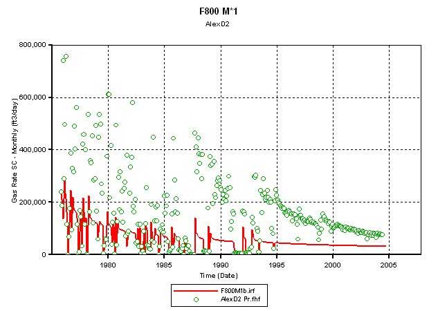
Figure 5b--Calculated production vs. actual production, fracture permeability 800 md.
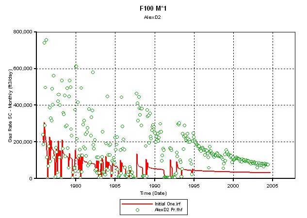
Figure 6--Calculated production vs. actual production, matrix permeability 4 times that of core-plug-based value. Use Matrix K multiplier: Frac phi = 0.35, K =400 md, Mat K*4.
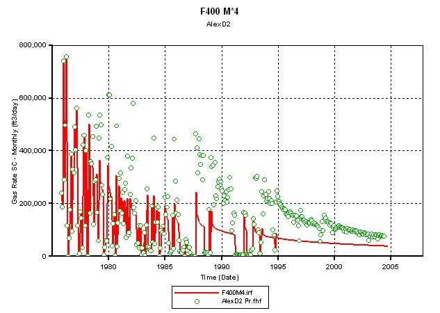
Figure 7--Calculated production vs. actual production, matrix permeability 6 and 8 times that of core-plug-based value. Use Matrix K multiplier Frac phi = 0.35, K =800 md, length = 660 feet, Mat K*8. Sim OGIP = 1859.2 mmscf.
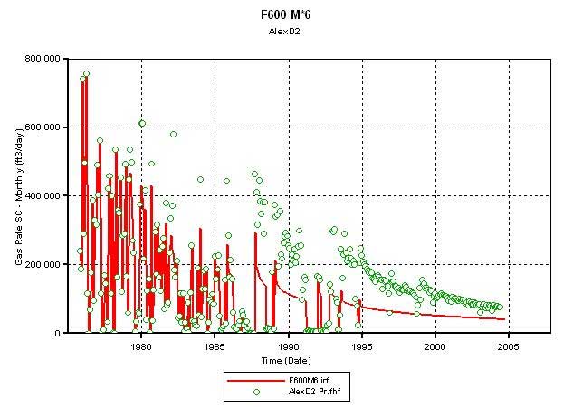

Figure 8--Relative permeability tables from the matrix and the fracture.
|
|
|||||||||||||||||||||||||||||||||||||||||||||||||||||||||||||||||||||||||||||||||||||||||||||||||||||||||||||||||||||||||||||||||||||||||||||||||||||||||||||||||||||||||||||||||||||||||||||||||||||||||||||||||||||||||
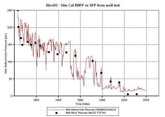
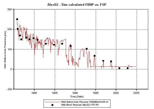
The Sw in the silt layers (till layer 94) was assumed to be at 0.8 to enable vertical gas flow through them. This resulted in an OGIP charge of 2.5 bcf in the simulated area as opposed to the volumetrically estimated OGIP of 1.86 bcf. The matrix permeability was maintained at 8 times that predicted by the plug-derived facies-based permeability-porosity correlations, while the fracture permeability was set at 800 md. Figure 9A shows that the simulator-calculated D2 output (red line) was able to match the historic production volumes (green circles). Lacking a regular record of water production, historic water production (blue line) was estimated by interpolating between available intermittent well test data. The simulator calculated water production (broken blue line) follows but is below the estimated historic trend. Average reservoir pressures were estimated by converting surface shut-in pressures to bottom-hole conditions, and are plotted as black squares. The simulator calculated average reservoir pressure is shown by the black line and it shows a good match till 1994. Some of the participating companies in this project have expressed concerns that the estimated bottom hole shut-in pressures underestimate the average reservoir pressure because in a tight reservoir such as the CG, a 72-hr shut-in test may not result in fully stabilized pressures at the surface. Figure 9B compares the simulator-calculated flowing bottom-hole pressure (FBHP) with the recorded flowing surface pressure (FSP). The FSP is not supposed to be equal to FBHP but for a shallow gas well, it is reasonable to expect FBHP to be close to FSP.
Figure 9a--Calculated production vs. actual production, use non-zero Sg in silt layers--Sw = 0.8 (till layer 94); Frac phi = 0.35, Frac K =800 md, Mat K*8.
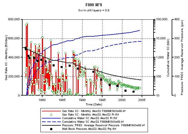
Figure 9b--Comparison of the simulator-calculated flowing bottom-hole pressure (FBHP) with the recorded flowing surface pressure (FSP).
The match obtained in Figure 9 required an OGIP charge of 2.5 bcf as opposed to the volumetric estimate of 1.86 bcf based on FWL level estimation from DST and production data. Thus, material balance (MB) calculations were conducted to approximate the OGIP and confirm if an OGIP charge of 2.5 bcf is reasonable or too high. Figure 10A plots P/z vs. cumulative production (Gp) for D2 since its inception to date. The plotted points align on a linear trend which results in a MB-OGIP of 1.82 bcf. However in 1991, Alexander D3 (called D3)--an infill Chase well was drilled in the same Section as D2. Figure 10B plots the post 1992 P/z vs. Gp data from D2 in order to eliminate interference effects, if any, from the D3. The points, again, show a linear trend though different from that shown in Figure 10B. The OGIP charge calculated using the Figure 10B trend is 2.27 bcf. Thus, using only the P/z vs. Gp data from D2 that pre-dated the D3 well, it is not unreasonable for the drainage area around D2 to carry an OGIP charge of around 2.3 bcf.
Figure 10a--P/z vs. cumulative production, all data. Simulation OGIP = 2505.7 mmscf. Volumetric OGIP = 1864 mmscf.
Material balance formulation:
P/z = Pi/zi - (Pi/zi)*(Gp/G)
Total gas reserves:
G = 1,828,945 mcf
Pi/zi = 238 psi
Gp = 1,659,456 mcf
RF = 0.91
Figure 10b--P/z vs. cumulative production, removing post 1992 data. Simulation OGIP = 2505.7 mmscf. Volumetric OGIP = 1864 mmscf.
Material balance formulation:
P/z = Pi/zi - (Pi/zi)*(Gp/G)
Total gas reserves:
G = 2,271,279 mcf
Pi/zi = 227.12 psi
Gp = 1,659,456 mcf
RF = 0.73
Figure 11 plots the bottom hole shut-in pressures, estimated from surface shut-in tests, for the 9 wells around and including D2. The pressures march almost in lock-step from 1975 to date. The Chase infill wells were drilled around 1992, and a change in the slope of the reservoir pressure decline occurs around this time raising questions about interference with the CG wells.
Figure 11--Bottom-hole shut-in pressures.
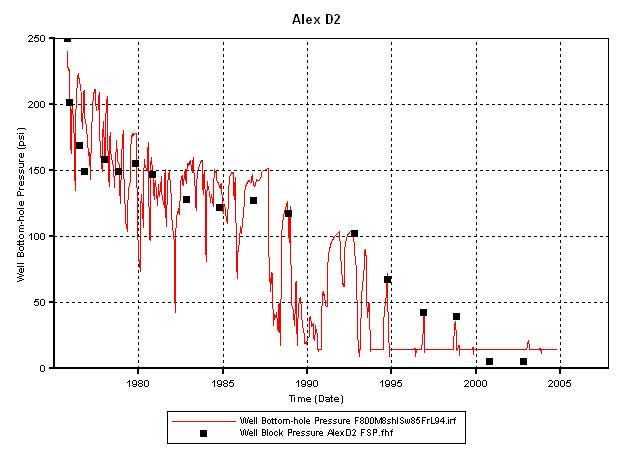
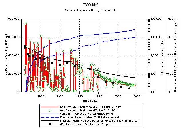
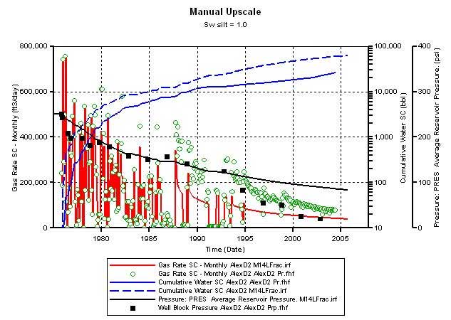
Figure 12 displays the results of the simulation run where the Sw in the silt layers was increased to 0.85 (from 0.8). This resulted in an OGIP charge of 2.34 bcf as opposed to 2.5 bcf when the Sw in the silt layers was set at 0.8. This newly calculated OGIP is closer to that (2.27 bcf) estimated from MB using pre-1992 P/z and Gp data from D2. Figure 12A shows that the simulator-calculated gas production at D2 traces the historic trends expect after 1994. Even after 1994, the simulator-calculated gas production is close to that recorded for D2. The water production from simulation output still trails the estimated water production history. Figure 12B shows that a good match is obtained between the simulator-calculated FBHP (red line) and the FSP (black squares) from the shut-in test data.
Figure 12a--Calculated production vs. actual production--use non-zero Sg in shale layers--Sw = 0.85 in shale layers; frac phi = 0.35, K =800 md, Mat K*8.

Figure 12b--Comparison of the simulator-calculated flowing bottom-hole pressure (FBHP) with the recorded flowing surface pressure (FSP).
To get a better match with the estimated water production history, the hydraulic fracture around D2 was vertically extended to layer 94 (Figure 13A) from layer 91 (Figure 13B). Extending the reach of the fracture resulted in a match with the estimated water production history (Figure 14). Thus, a reasonable match of the production and pressure is obtained for D2 when the matrix permeability in its drainage is set at 8 times that predicted by plug-based facies-specific permeability-porosity correlations and when the OGIP charge is set at 2.3 bcf. Plug-based permeability measurements represent a biased sampling because the plugs are normally taken from areas with least heterogeneity and represent only an infinitesimal fraction of the reservoir volume drained by the well. The fluid flow in the drainage area of the well may be affected by different scales of heterogeneities that are not sampled by the plugs. Thus, it is necessary to cross-check if the use of an effective permeability that is eight times that measured on core plugs is reasonable.
Figure 13a--Match water production--extend fracture to Layer 94. Frac phi = 0.35, K =800 md, Mat K*8, Sw = 0.85 in silt layers.
Figure 13b--Original fracture description.
Figure 14a--Calculated production vs. actual production--to match match water production, extend fracture to Layer 94; Frac phi = 0.35, K =800 md, Mat K*8, Sw = 0.85 in silt layers.
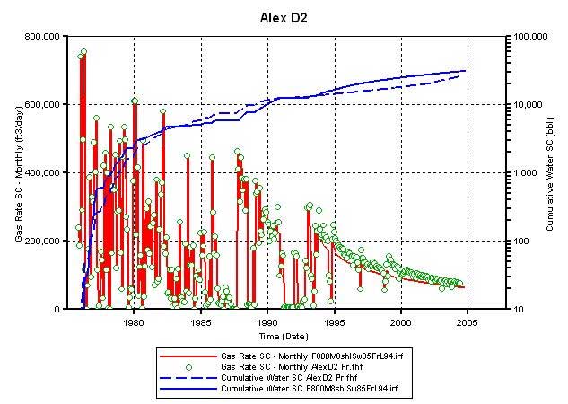
Figure 14b--Comparison of the simulator-calculated flowing bottom-hole pressure (FBHP) with the recorded flowing surface pressure (FSP).
The 3D static cellular models for the two simulation exercises were constructed in similar fashion with each cell in the model being populated with lithofacies, porosity, permeability, and water saturation (Sw) properties. The models were then upscaled by reducing the number of layers and estimating new properties for the new coarser layers for all except the discrete lithofacies property. Upscaling is required in larger models for more efficient simulation. To investigate the degree to which the model can be upscaled without compromising the simulation output, the fine scale model was reduced to 896 cells by reducing the number of layers to fourteen layers (Figure 15), to the marine and nonmarine half-cycle scale. Each of the fourteen layers is a marine or nonmarine half-cycle of the seven marine-nonmarine sedimentary cycles in the Council Grove reservoir.
Figure 15--New model has only 14 layers.
The fine scale model was upscaled to 14 layers (Figure 15) manually. Porosity was weighted by thickness for averaging, while Sw was pore-volume weighted. The horizontal K was thickness-weighted for averaging while the vertical K was thickness-weighted for harmonic averaging. As a result of this upscaling, none of the two layers from the bottom has a starting Sw = 1.0 though constituent fine-scale silt layers were assumed to be at Sw = 1.0. The simulator calculated OGIP was 1.8 bcf (similar to that obtained in the starting volumetric model). Figure 16 compares the results from the upscaled model with the fine scale model, and shows that the simulator calculated gas production (Figure 16A) using the 14-layer model is close to that of the 96-layer model (Figure 16B). Thus, it appears that an upscaled model is effective in simulating the complex drainage area around D2. A similar upscaling experiment was carried out assuming that the silt layers in the underlying fine-scale model were at Sw = 0.85 (Figure 17). The simulator calculated OGIP was 2.3 bcf (Figure 17A). The resulting gas and pressure match was similar to that obtained using corresponding fine-scale models (Figures 17B and 17C).
Figure 16a--Calculated production vs. actual production in new 14-layer model. Simulator OGIP = 1857.6 mmscf. This model has silt Sw = 1.0.

Figure 16b--Calculated production vs. actual production for original 96-layer model for comparison to new coarser model.
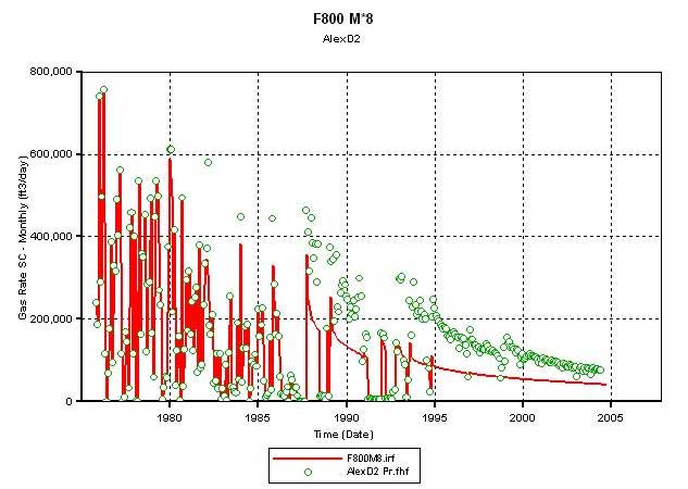
Figure 17a--Calculated production vs. actual production 14-layer model. This model has silt Sw = 0.85.
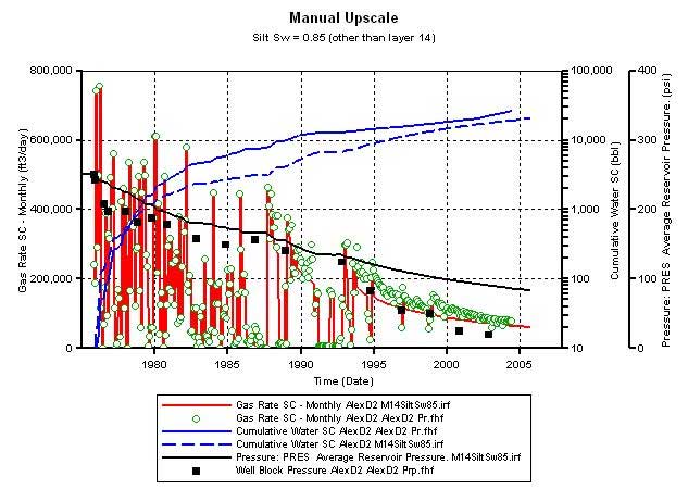
Figure 17b--Similar to figure 14a, calculated production vs. actual production--to match match water production, extend fracture to Layer 94; Frac phi = 0.35, K =800 md, Mat K*8, Sw = 0.85 in silt layers.
Figure 17c--Similar to Fig. 12a, calculated production vs. actual production--use non-zero Sg in shale layers--Sw = 0.85 in shale layers; frac phi = 0.35, K =800 md, Mat K*8.
Upscaling operations (Figures 18 to 20) were performed in Petrel for porosity and water saturations using an arithmetic average method. Permeability was upscaled in Petrel using the applications-tensor option that generates permeability for the coarse layers in the x, y, and z directions. Since all layers have continuous properties, tensor upscaling results are the same as arithmetic averaging. Figure 21 compares the simulated results using the Petrel-upscaled and manually upscaled model. The gas production calculated for D2 and the estimated average reservoir pressures compare well between these two models.
Figure 18a--Upscaling in Petrel--15 Horizons, 14 Zones (A1_SH, A1_LM, B1_SH, ....). Fine model: Facies based log phi_corr at one-foot scale; coarse model: Arithmetic average.
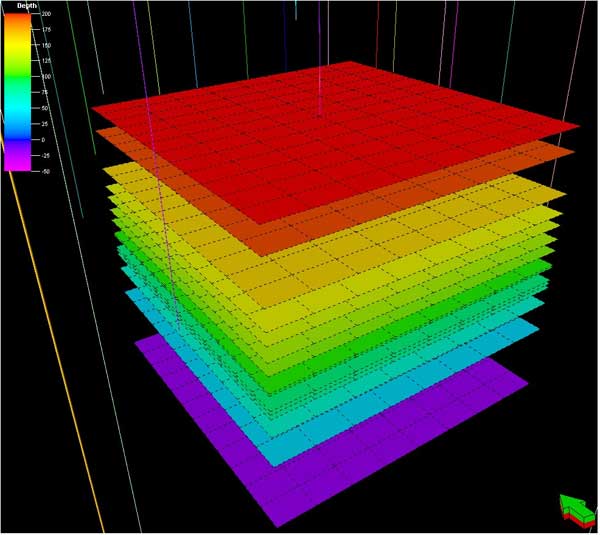
Figure 18b--Fine Model (233 one-foot layers)--porosity 0-20% scale. Fine model: Facies based log phi_corr at one-foot scale; coarse model: Arithmetic average.
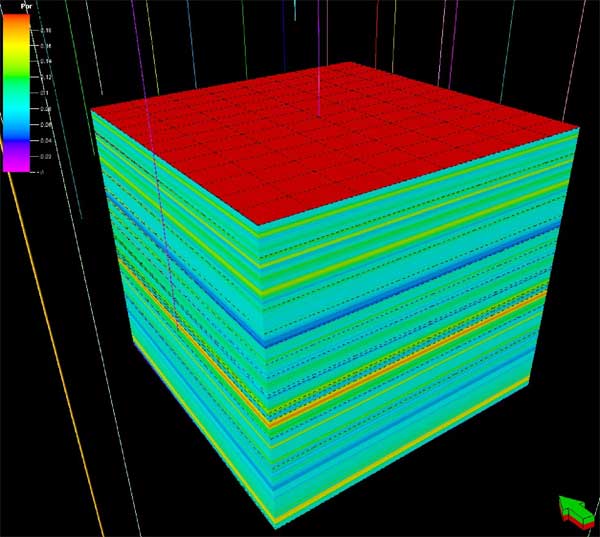
Figure 18c--Coarse Model (14 layers A1_SH, A1_LM, B1_SH, ....)--porosity 0-20% scale. Fine model: Facies based log phi_corr at one-foot scale; coarse model: Arithmetic average.
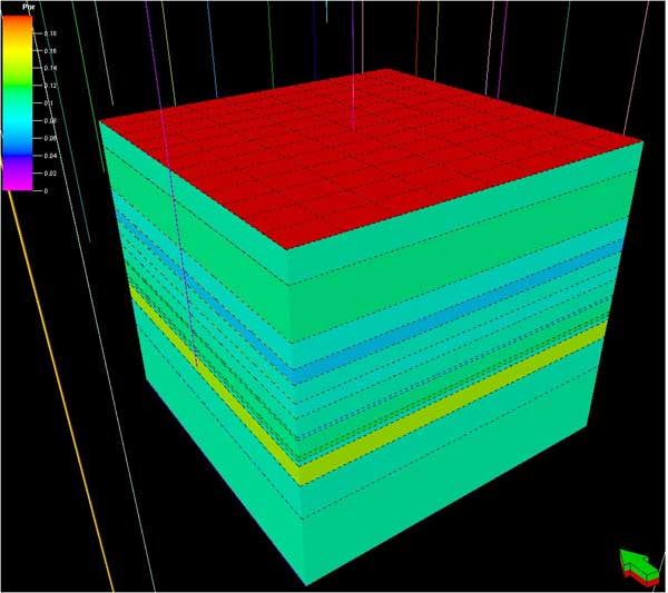
Figure 19--Permeability--All scales 0.001-100md. Fine model: matrix plug k from log phi_corr, facies, and property transforms. Coarse model: Petrel Tensor upscaling. 19a--Kij Fine Model.
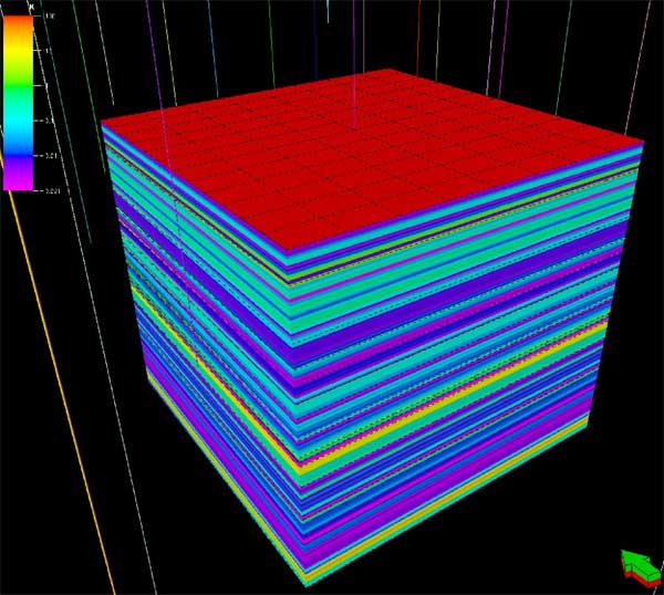
Figure 19b--Kij Coarse Model.
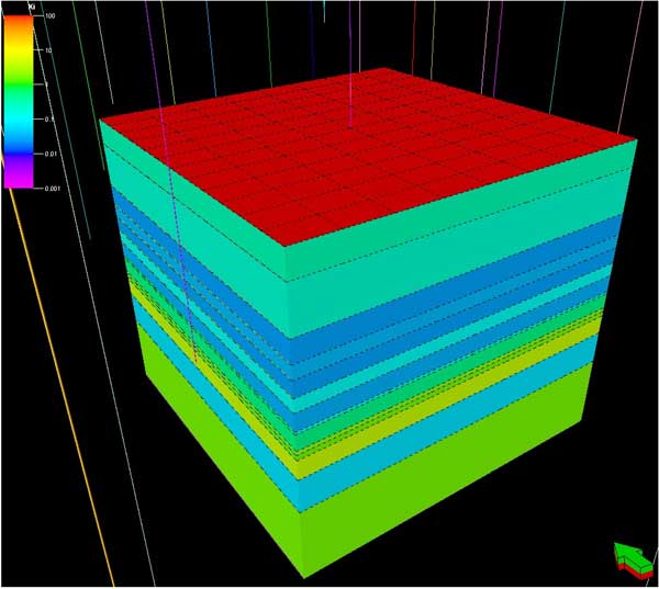
Figure 19c--Kij_8X.
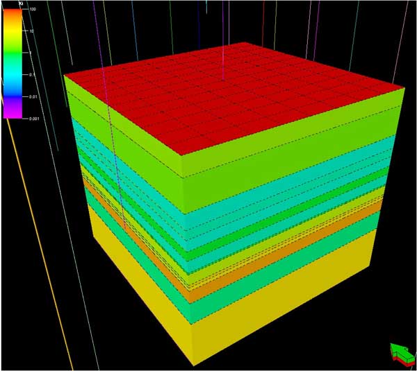
Figure 19d--Kz Coarse Model.
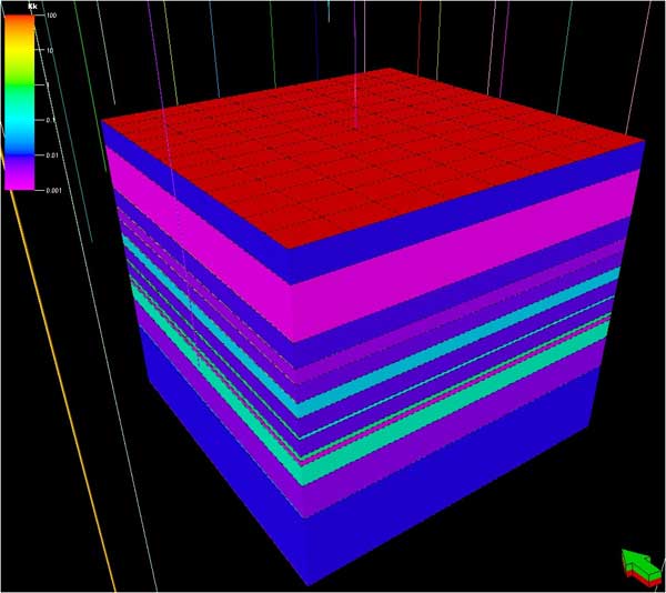
Figure 19e--Kz_8X.
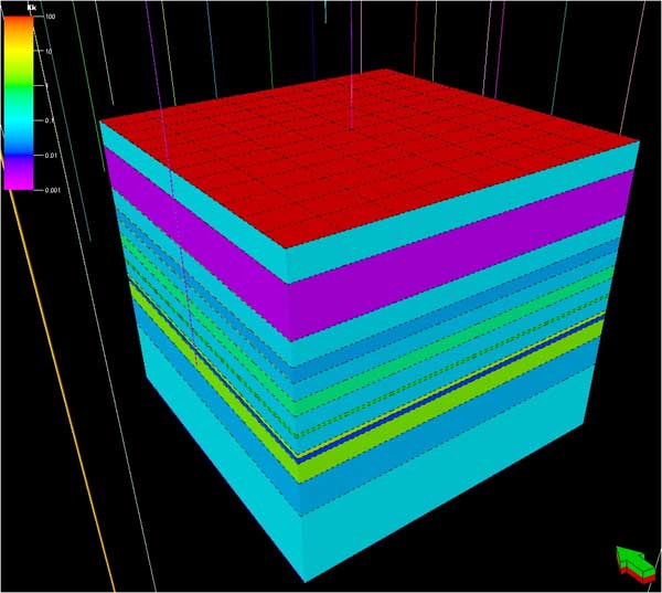
Figure 20a--Water Saturation--Sw Fine Model.
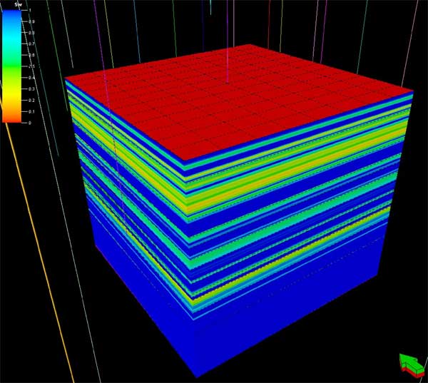
Figure 20b--Water Saturation--Sw Coarse Model.
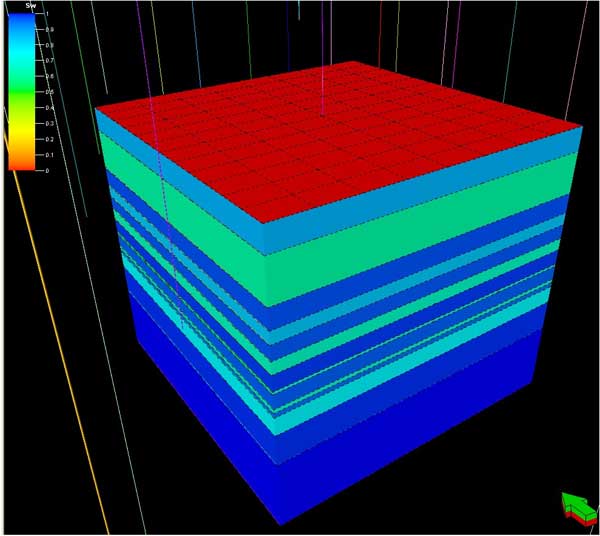
Figure 21a--Calculated production vs. actual production of model upscaled using Petrel to 14 layers--silt Sw = 1.0. OGIP = 1818.9 mmscf.
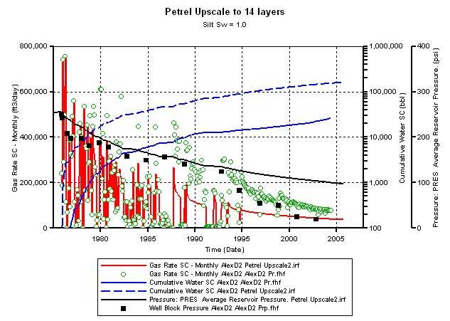
Figure 21b--Calculated production vs. actual production of manually upscaled model. OGIP = 1857.6 mmscf.
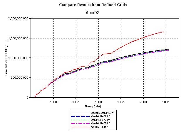
The issue of grid refinement effects on simulator calculated results was also investigated. Refined grid experiments were carried out on the up-scaled 14-layer model. Three types of refinements (Figures 22A, 22B, and 22C) were carried out ranging from grid cell sizes of 132 feet by 132 feet to 66 feet by 66 feet. The original grid cell size used in all the previously discussed simulation runs was 660 feet by 528 feet. Figure 23 compares results from the refined grid experiment. The red curve is historic production. The black line is that obtained using un-refined 14-layer model. The broken blue, green, and magenta lines represent output from the 3 refined grids. It appears from the above results that grid refinement ranging from 660 feet by 528 feet to 66 feet by 66 feet does not affect simulator output significantly to offset K increase in Council Grove to history match Alex D2 production.
Figure 22a--Refinement 1 (132 feet by 132 feet). Unrefined grid size: 660 feet along X and 528 feet along Y.
Figure 22b--Refinement 2 (132 feet by 132 feet). Unrefined grid size: 660 feet along X and 528 feet along Y.
Figure 22c--Refinement 3 (66 feet by 66 feet). Unrefined grid size: 660 feet along X and 528 feet along Y.
Figure 23--Calculated production vs. time for the models.
Dubois, M.K., Byrnes, A.P., Bohling, G.C., Seals, S.C., and Doveton, J.H., 2003, Statistically-based lithofacies predictions for 3-D reservoir modeling: an example from the Panoma (Council Grove) Field, Hugoton Embayment, southwest Kansas (abs.): American Assoc. of Petroleum Geologists, 2003 Annual Convention, vol. 12, p. A44, and KGS Open-file Report 2003-30. [Available online]
Kansas Geological Survey, Energy Research
Placed online May 12, 2005
Comments to webadmin@kgs.ku.edu
The URL for this page is HTTP://www.kgs.ku.edu/PRS/publication/2004/OFR04_66/index.html