South-central Kansas CO2 Project CO2 Sequestration Lunar and Solar Tidal Pressure

Work is partially supported by the U.S. Department of Energy (DOE) National Energy Technology Laboratory (NETL) under Grant Number DE-FE0006821.

The continuous pressure monitoring in the lower Arbuckle was set up because a large rate and high volume brine disposal in the area is believed to be responsible for the induced seismicity. "The assumption in the case of the testing in the Arbuckle is that the observed pressure is being transmitted at depth in the basement where faults are critically stressed, requiring a small force to move. To date the vast majority of earthquakes have occurred in the shallow basement." Quarterly Report-19, 2016. Trilobite Testing of Hays Kansas installed the pressure gauge in the Wellington KGS 1-28 at about 5020 feet depth from surface. The instrument is programmed to sample every second with an accuracy of 0.1 psi. About a week of pressure data is sent to KGS as a Comma Separated Values (CSV) file.

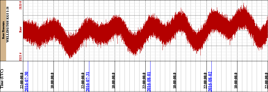
A Java computer program was developed to analyze the pressure data from the Wellington KGS 1-28 to understand the pressure changes, to remove solar & lunar Tidal pressures along with barometric pressure changes. The idea is that if you can remove or explain the natural every day influences you are left with the geological influences and maybe you might be able to identify fluid movement due to brine injection, micro quake swarms, etc. Figure 1 is an illustration of the raw pressure measurement in psig units over a 4 day period, 30 July to 2 August 2016.

The computer program will filter the noise from the raw pressure data, compute the lunar & solar tidal pressures along with the barometric pressures influence, and then subtract that from the raw pressure data. In an ideal situation if these are the only pressures influencing the pressure measurements then the pressure data should result in a straight line.

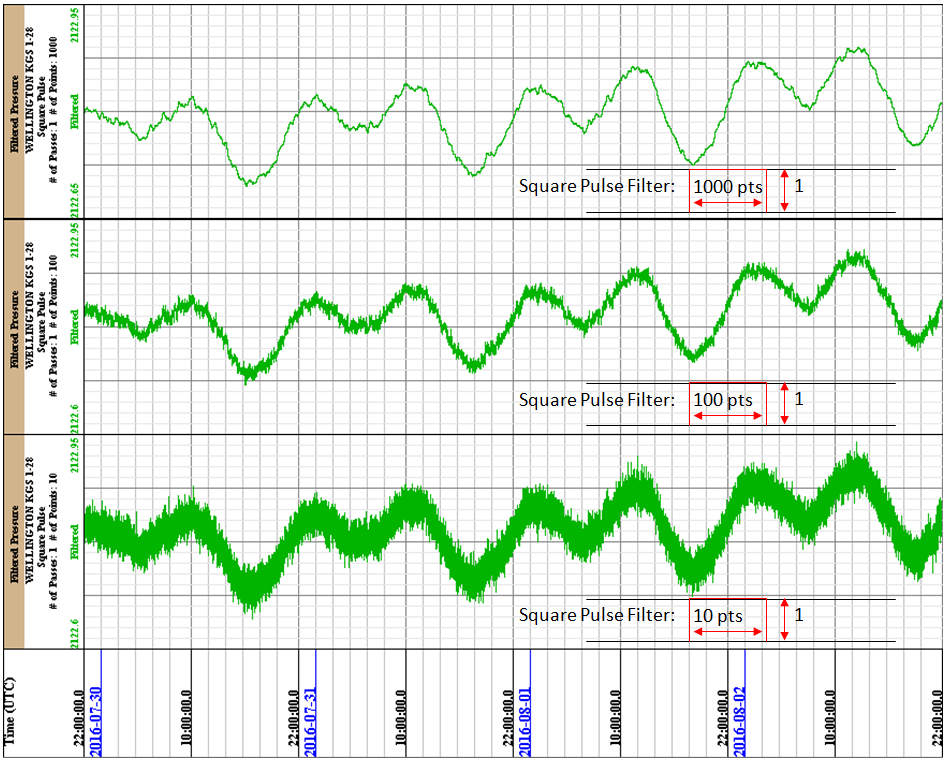
The first step was to filter out as much of the measurement noise in the Raw Pressure data. Playing with a simple square pulse filter of varying width gives varying improvements to the Pressure data, see figure 2. The best result was the 1000 points (1000 seconds) square pulse applied to the raw data. This method removed most of the noise, without removing signals that may be of interest down the line. You can see the lunar and solar cycle in the pressure wave as well as "noise" on top of that signal or is it barometric pressure or something else.

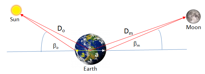
²It is well known that the sinusoidal water level variations observed in open wells are directly related to lunar & solar tidal influence. It is also believed that the tidal effects are related to the characteristics of the formation and to the fluid contained in the formation. The lunar & solar attraction of the earth generates a state of stress on the earth’s surface which induces a radial deformation of the earth. As the gravitational force of attraction between two masses is inversely proportional to the square of the distance between these two masses, the potential derived from this force will be inversely proportional to the distance between the two masses. In Bredehoeft¹ he attributes to Love³ (pg 52) that the tide generating potential W may be approximated with sufficient accuracy as a spherical harmonic of second degree,

W = 0.5 * (GM_b/D_b)(a/D_b)² (3 cos²β_b -1)       (1)

where
G is the Gravitational Constant = 6.67408 X 10^-11 [m3]/{[kg][sec2]}
M_b - Mass of the body
D_b - Distance between earth and body
a - Earth Radius = 6.371 X 10⁶ [m]
β_b - angle between earth and body

Expanding cos(β_b) with respect to earths latitude and longitude,

cos(β_b) = sin(λ_e) sin(λ_b) + cos(λ_e) cos(λ_b) cos(ωt - φ_b )       (2)

where
β_b - angle between earth and body
ω - frequency of the Earth’s rotation = 1.1600804 X 10^-5 [Hz]
λ_e - latitude of the Wellington KGS 1-28 = 37.3194833 degrees
λ_b - latitude of the body, which is "moving" up and down with respect to earth with time
φ_b - longitude of the body, which is "moving" around earth with time

Lunar tidal influence is about twice as strong as the solar tidal influence, but not insignificant as some authors imply. Using the tide generating potential constant (GMb/Db) (a/Db)2 for both the moon and the sun,

M_m - Mass of the moon = 7.34767309 X 10²² [kg]
D_m - Average distance between earth and moon = 3.84402 X 10⁸ [m]

M_o - Mass of the sun = 1.989 X 10³⁰ [kg]
D_o - Average distance between earth and sun = 1.495979 X 10¹¹ [m]

	Moon	Sun
(GMb/Db)(a/Db)2	3.504275 [m/sec]2	1.69404 [m/sec]2

Bredehoeft¹ states that the dilatation in an aquifer will depend not only on the tidal strain but also on the effect of change in internal fluid pressure produced by the tidal dilation. The aquifer will be subjected to tidal strains latitudinal and longitudinal directions that are almost entirely determined by the elastic properties of the earth as a whole. Love³ (pg53) showed that the dilation can be related to the disturbing potential by introducing a fourth Love number, F(r), where

θ = F(r) * (W / g)

Takeuchi⁴ evaluated F(r) by numerical calculations indicating that near the earth’s surface the dilatation is given by

θ = (0.49 / a) * (W / g)       (3)

where a is the earth’s radius, g is the acceleration due to gravity (9.8 m/sec2) and W is the lunar & solar tide generating potential. Bredehoeft continues to derive the effects of the dilation as change in pressure of the earth tide in an aquifer system and shows that the earth tide P is,

P = ρgh = θ / (Cw φ)       (4)

where ρ is the density of the fluid in the borehole, g is the acceleration due to gravity and h is the height of the fluid above the aquifer, φ is the porosity of the aquifer, θ is the volumetric strain at the surface of the earth, C_w is the compressibility of the water. The compressibility of the rock itself was neglected because Bredehoeft assumed that the change in rock matrix volume was small compared to that of the water volume.

The lunar & solar tide generating potential, W_b, equation used in the Java Web App is as follows,

W_b = 0.75 * [GM_b/D_b] * [a/D_b]² * {
     (3*cos(2*λ_b) -1) * (3*cos(2*λ_e) -1) /12.0       Long term cycle
      + sin(2*λ_b) * sin(2*λ_e) * cos(ωt - φ_b - φ_corr)      Diurnal ~1 day cycle
      + cos² (λ_b) * cos²(λ_e) * cos[2*(ωt - φ_b - φ_corr)]}      Semi-diurnal ~1/2 day cycle

where
G is the Gravitational Constant = 6.67408 X 10^-11 [m3]/{[kg][sec2]}
M_b - Mass of the body
D_b - Distance between earth and body varying with time
a - Earth Radius = 6.371 X 10⁶ [m]
ω - Frequency of the Earth’s rotation = 1.1600804 X 10^-5 [Hz]
λ_e - Latitude of the Wellington KGS 1-28 = 37.3194833 degrees
λ_b - Latitude of the body, which is varying with time, and computed from the declination [degrees].
φ_b - Longitude of the body, which is varying with time, computed from right ascension.
φ_corr - Correction angle due to the "starting time" of pressure data file.

The total generating potential W is the sum of lunar (W_m) and solar (W_o) potentials, i.e. W = W_m + W_o. Substituting the total generating potential W into equation (3) and then into equation (4) gives the pressure due to earth tide as follows,

P = (0.49 / a) * (W / g) / (C_w φ)

where in Wellington KGS 1-28 at 5020 feet below the surface in the Arbuckle formation the water temperature is 133.01 [degrees F] from the Temperature Log, log date 3 March 2011 by Halliburton, gives a water compressibility (C_w) of 0.4437 [1/GPa] and the Porosity of the aquifer (φ) is about 0.13 [PU].

The apparent latitude and apparent longitude of the Moon and Sun is computed using the equations from ⁵"How to compute planetary position" by Paul Schlyter.

The slope is computed by taking the first 1000 points (1000 seconds) and computing the average and then taking the last 1000 points (1000 seconds) and computing the average, then visually modifying the starting pressure and ending pressure with respect to the filtered pressure curve after the lunar & solar pressure is subtracted to represent the slope of the filtered pressure data.

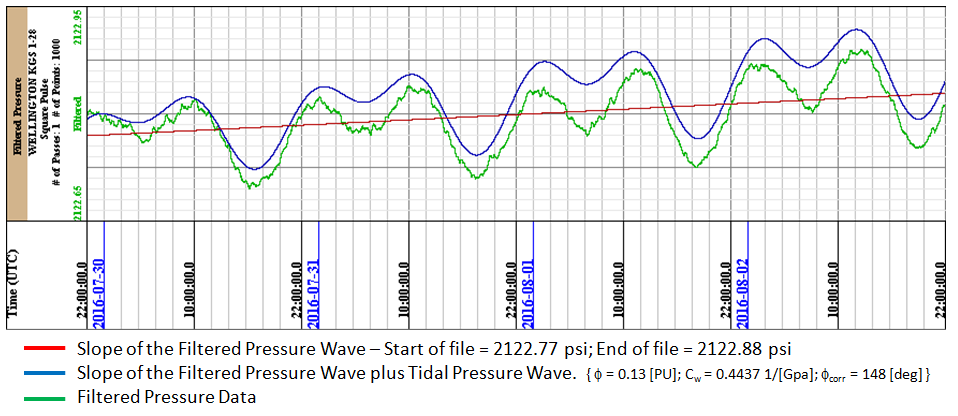
The last step in the program is to subtract the lunar & solar tidal pressure wave from the filtered pressure wave, which should show the data to be linear. The data is not totally linear, which suggest there is something else pulling and pushing the pressure curve. For this data set a barometric pressure was measured at Strother Field Airport, Hackney, Kansas, which is 24.2335 miles to the Southeast of the well. If there were major pressure fronts or large storms then the barometric pressure from Strother Field Airport should suggest the changes in the deviation of the filtered pressure wave after the lunar & solar wave is subtracted. The pressure change from the surface pressure and the pressure measured at the pressure sensor is just the weight of the water column above the sensor, i.e.,

P_sensor = P_atmosphere + ρgh.

where ρ is the density of the fluid in the borehole g is the acceleration due to gravity (9.8 m/sec2) and h is the height of the fluid above the pressure sensor.

We do not have the exact height of the water column above the pressure sensor, so the only way to incorporate the barometric pressure influence at the pressure sensor is to estimate what the measured pressure data should be at the sensor. The atmospheric pressure at Wellington KGS 1-28 is about 14.11 psi from the calculation of ideal altitude versus pressure curve. Ideally if the lunar & solar pressure curve is subtracted from the measured data then the measured data should be a straight line. It is basically a straight line in the image below (figure 5) but there are deviations.

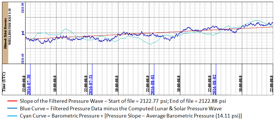
A pressure curve is constructed by adding the barometric pressure measured at Strother Field Airport with the difference of the Pressure Slope and 14.11 psi the average ideal barometric pressure at this elevation and overlaying that on the measured data. It can be seen that there is some comparison with the measured data. Ideally if the barometric pressure is measured at Wellington KGS 1-28 then the computed barometric pressure should line up exactly with the linear pressure curve and any deviations from that would be other geological effects, i.e. fluid movement, etc.

References:

1) Response of Well Aquifer Systems to Earth Tides by John D. Bredehoeft, Journal of Geophysical Research, Vol 72, No 12 June 15, 1967.

2) The Earth Tide Effects on Petroleum Reservoirs, Thesis submitted to the Department of Petroleum Engineering of Stanford University by Patricia C. Arditty, May 1978

3) Love, A. E. H., Some Problems o] Geodynamics, 180 pp., Cambridge University Press, Cambridge, 1911, https://archive.org/details/cu31924060184367

4) Takeuchi, H., On the earth tide of compressible earth of variable density and elasticity, Trans. Am. Geophys. Union, 31, 651-689, 1950.

5) How to compute planetary positions by Paul Schlyter http://astro.if.ufrgs.br/trigesf/position.html

Author: John R. Victorine jvictor@kgs.ku.edu The URL for this page is http://www.kgs.ku.edu/Ozark/JAVA_SRC/PSI_Tides/index.html