Kansas Geological Survey, Current Research in Earth Sciences, Bulletin 253, part 2
Prev Page--Introduction, Background || Next Page--Fracture System, Lineaments
![]()
![]()
![]()
Kansas Geological Survey, Current Research in Earth Sciences, Bulletin 253, part 2
Prev Page--Introduction, Background ||
Next Page--Fracture System, Lineaments
![]()
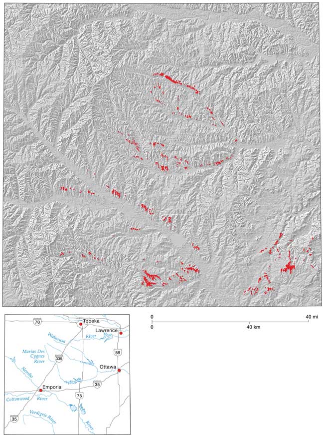
The term "high-level" chert gravel here connotes gravel deposits that are topographically higher than the deposits being formed at present by streams or that reside in modern low-level stream terraces. The locations of the high-level gravels in the "experimental" area are shown in fig. 6. Of course, the present streams transport chert pebbles (among other materials) and locally extensive gravel deposits occur in modern streams. Importantly, the properties of the modern streams and perhaps their floodplains may be similar in general form to those of the ancient streams that deposited the high-level chert gravels.
Figure 6--Mapped distribution of high-level chert gravels mapped in the "experimental area" superimposed on the shaded-relief map.
The high-level chert gravels provide evidence of the gradients of ancestral streams. As described in a related article by Merriam and Harbaugh (2004), the chert fragments have been derived through weathering of chert-bearing Permian limestones that crop out in the Flint Hills. The chert, being relatively insoluble by comparison with the limestone, tends to be concentrated in soils and lag gravels before being transported. Prolonged solution of the limestones has provided abundant chert-bearing gravel for transport by east-flowing ancient streams that were ancestral to the present streams. Although they consist mostly of chert, some of the high-level gravel deposits have a matrix of reddish clay, suggesting that clay may have been part of the lag deposits and transported along with the chert fragments.
The chert fragments in the present high-level gravels were assuredly derived from Permian limestones in the Flint Hills and not from limestones in the Pennsylvanian sequence east of the Flint Hills over which the gravels have been deposited. The Pennsylvanian limestones contain relatively little chert, whereas the Permian limestones in the Flint Hills generally have a high proportion of chert (Merriam and Harbaugh, 2004, fig. 4). Furthermore, some of the fusulinids in the chert fragments are Permian in age, and not Pennsylvanian (Merriam, 1963).
Attributing the high-level chert gravels to deposition by streams is problematic. First, even in the best exposures such as pits where they have been quarried for road material, the gravels lack the most rudimentary aspects of stratification, including cross stratification.
The sizes and shapes of the chert particles are also puzzling. Most exhibit a degree of rounding, but many are relatively angular (Merriam and Harbaugh, 2004, fig. 5), and the gravel deposits generally are poorly sorted by size, with large and small particles jumbled together in disorder, the largest being about 15 cm across. Thus, although the high-level chert gravels may not be typical stream-gravel deposits, it is difficult to devise an alternate means by which they might have been transported.
Transport of chert-bearing gravels from the Flint Hills by east- or southeast-flowing streams has been going on for a long time. It is occurring today, and presumably has taken place during the Quaternary (Pleistocene) and Tertiary (Neogene), and perhaps even earlier. The time span is problematical, for there is no firm dating method for these deposits. It is reasonable, however, to presume that streams flowing over low gradients toward the east and southeast were part of an ancestral drainage system that deposited the gravels, and the upland gravels that we see today are remnants left high and dry as the streams cut down.
Mapping of the high-level chert gravels suggests that there are at least two separate levels of high-level chert gravels, namely a younger "lower" high-level chert gravel, and an older "upper" high-level chert gravel (Aber, 1992). In places, the remnants of these gravels are a meter or more thick, although the thicknesses are extremely variable and are difficult to measure because of poor exposures. The age difference between the "upper" and "lower" gravels is problematical, but presumably the "lower" gravels were deposited considerably later than the "upper" gravels.
Some of the "upper" high-level chert gravels occur on the tops of hills on interstream divides. Although these high-level chert gravels have been largely removed by subsequent erosion, they are presumed to have once been more widespread in eastern Kansas. Furthermore, older and higher high-level chert gravel deposits may have been present, but if they existed, no remnants have been identified. Given that the gravels were deposited by streams, however, it is unlikely that they formed sheetlike deposits that extended more or less continuously over large areas, and we may presume that they formed along successive floodplains of ancient streams.
An assumption that needs to be weighed carefully involves the three-dimensional positions of the chert gravels. If they are fluvial deposits, the surfaces on which they rest must be ancient land surfaces, or more properly, they must be the bedrock surfaces over which streams flowed that deposited the gravels. This is a critical assumption. Wherever the high-level chert gravels have been preserved, remnants of the old bedrock surfaces also have been preserved. If these remnants can be linked appropriately, the gradient or general slope of the ancient landscape over which the ancient streams flowed can be reconstructed.
However, the fact that only scattered remnants of these ancient fluvial deposits have been preserved is problematical. The present-day geographic distribution in the experimental area (fig. 6) suggests that the gravels probably were more widespread in the past, so the remnants preserved today probably represent only a portion of the gravel's former aggregate areal extent. We may presume, however, that the ancient deposits formed on low-lying surfaces along ancient drainage ways and did not form widespread blanket deposits continuous over large areas.
Because the high-level chert gravel deposits are relatively small in area and vegetation cover is extensive, it stands to reason that probably remnants of chert-gravel deposits that have not been located or mapped do exist. The sparse distribution of remnants of high-level chert gravels raises the question as to the efficacy of the mapping. Could there be other remnants that are present but have not been detected in mapping? The answer is a guarded yes. The favorite places to look for chert fragments are on the tops of hills, in fields, or in ditches along roadsides. The gravels have been quarried for road material in places where they are thick, and of course old quarries are relatively easy to locate.
The question is whether improved mapping would provide substantially more evidence. If more high-level chert deposits could be located, it would be useful to know about them. On the other hand, the conclusions reached here probably would not be seriously altered, although knowledge of more gravel deposits might enable us to refine our estimates of the ancient stream gradients and general directions of flow.
Mapping the elevations of the high-level chert gravels involves coordinating their locations with the DEM data. The elevations of high-level chert-gravel deposits of equivalent age must necessarily become progressively lower toward the southeast if southeastward-flowing streams deposited them, suggesting that reconstruction of former stream gradients can be made with relative confidence.
We note that because data in the DEM files have been obtained by digitizing elevations from topographic maps, the elevation data in figs. 5, 10, and 11 are surrogates for conventional topographic maps, although they present information in different graphic form.
Ascertaining old stream gradients involved repeated trials with different assumptions about the theoretical elevations and gradients of these ancient streams and comparing them with the gradients and elevations of actual remnants of the gravels segregated into "upper" and "lower" gravels. The locations of the actual gravels are known from geologic mapping, and the DEM files provide their elevations. In a succession of trial-and-error GIS "experiments," we generated theoretical surfaces on which the "upper" gravels could have been deposited and then located places where these theoretical gravels could accord with the present topography. We experimented with dozens of different gradients and slope directions until we eventually obtained a combination of gradient and slope that provides a best match between locations of the theoretical deposits and locations of actual deposits. We conducted a similar series of experiments for the "lower" gravels. In the end, we decided to represent the two theoretical surfaces with two parallel planes separated by an interval of 24.5 m, thus providing identical stream gradients and slope directions for the hypothetical "upper" and "lower" gravels.
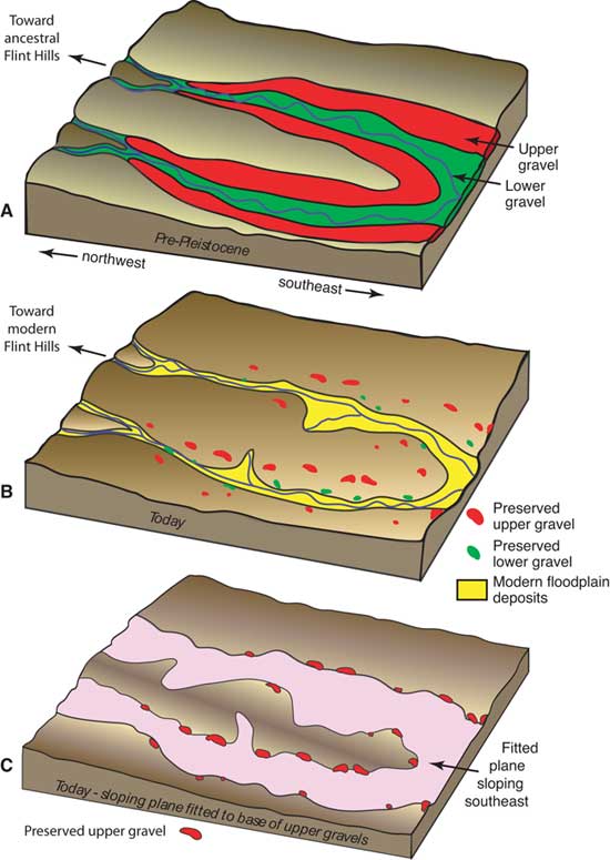
The procedure employed in the experiments is simple in principle, although the GIS operations are challenging. The procedure is illustrated schematically in fig. 7, which consists of three related block diagrams that show a hypothetical part of the study area. The upper diagram (fig. 7A) represents the geologic past when the younger "lower" high-level chert-gravel deposit was being formed, whereas the older "higher" deposit was partially preserved as an extensive terrace deposit. Figure 7B represents the area today, with scattered remnants preserved of both the "upper" and "lower" deposits. Figure 7C also represents the area today, but differs in that a theoretical sloping plane has been fitted to the base of the remnants of the "upper" deposit. The elevation, slope gradient, and slope direction of the fitted plane are interpreted as approximations of the gently sloping alluvial plains on which the "upper" deposit was formed.
Figure 7--Schematic diagrams illustrating fitting of theoretical gravel deposit to actual high-level terrace-gravel deposits. Although no exact scale is implied, block diagrams represent an area about 40 km northwest-southeast with a topographic relief of about 60 m. A, Late Tertiary: Progressive erosion has created a broad alluvial plain (green) on which a younger "lower" high-level gravel deposit is forming. Older "higher" high-level gravel deposit has been preserved in part and forms an alluvial terrace (red). B, Today's topography (brown) on which remnants of lower and higher high-level gravel deposits (denoted by green and red) have been preserved. Modern alluvial plain is denoted by yellow. C, Today's topography and remnants of actual higher high-level gravel deposits (red) to which a gently sloping plane (pink) representing base of theoretical gravel layer has been fitted to coincide with elevation of actual deposits. (Note that lower high-level deposits (younger) are obscured because they lie beneath fitted plane). Fitted plane is interpreted as restoration of gradient and position of alluvial plain on which actual higher high-level gravel deposits formed.
As an end product of our experiments, the two theoretical gravel layers have been defined as bounded by planes that are parallel to each other (fig. 8). The thickness of each layer and the interval between them were added to become part of the definition. Because the two layers are parallel, the slope gradient and slope direction are identical for the planes, so that the only other parameters needed are the elevations of the planes at the "pivot point" (fig. 9) and the geographic coordinates of the pivot point. Given this information, the system of planes defining the upper and lower surfaces of each of the two layers is completely defined and GIS experiments with ArcInfo are feasible.
Figure 8--Schematic cross section showing manner in which two theoretical chert-gravel layers are superimposed on topography. Each layer is 8 m thick. Interval of 24.5 m separates base of upper layer from top of lower layer. Where either layer lies beneath or above present topography, it is omitted. Where layer touches present land surface, however, it is "preserved" (shown in orange) over vertical span that accords with layer's thickness. Thus, theoretical layer forms deposits that are "preserved" only where they are in contact with present land surface.
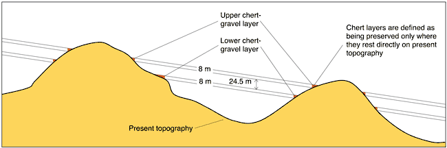
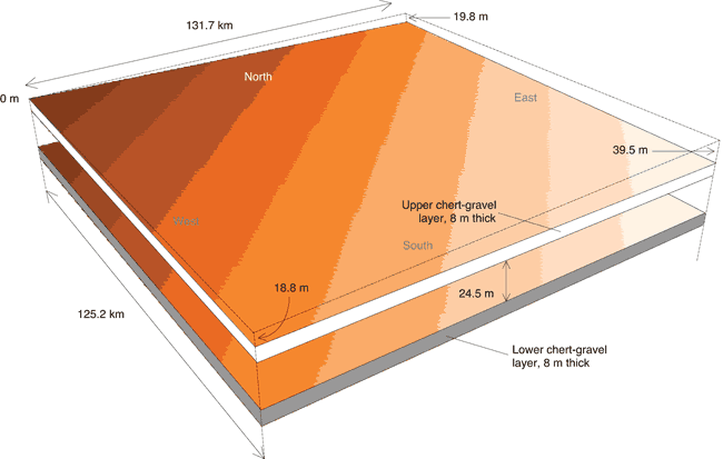
Figure 9--Schematic diagram showing two theoretical chert-gravel layers that slope southeastward from pivot in northwestern corner of area represented in diagram, which corresponds to experimental area outlined in fig. 3. Area is 131.7 km east-west, and 125.2 km north-south. Each gravel layer is 8 m thick and separation between them is 24.5 m. Upper layer is shown in white, and lower layer in gray. Layers slope uniformly 0.0015% to east and 0.0015% to south, with overall slope of 0.0021% southeast. With respect to pivot location in northwestern corner, each gravel layer is 19.8 m lower in northeastern corner, 18.8 m lower in southwestern corner, and 39.5 m lower in southeastern corner. Contour intervals are represented by bands of colors, each band corresponding to contour interval of 5 m.
As described in the Appendix using the GIS procedures employed in the study, entries for the parameters in experiments provide a high degree of flexibility. Two separate slope angles, one with respect to north-south and the other with respect to east-west, are entered for each of the theoretical gravel layers. This permits them to have separate slope gradients and slope directions if desired. Similarly, an individual thickness can be entered for each gravel layer. In keeping with this flexibility, the elevation at the pivot point must be supplied for the base of each of layer, so that the two layers need not be parallel in experiments.
In our experiments, various combinations of slope gradients, slope directions, thicknesses, separation intervals, and elevations at the pivot location were tried. The challenge was to determine what combination yielded the best accord between actual chert gravels and the theoretical surfaces. Although a simple objective, our study involved successive trials with a potentially vast number of possible combinations. Figures 8 and 9 illustrate the combination of assumptions that in the end yielded the best accord with the actual gravels.
Selecting a pivot location is a key initial step. We placed it in the northwestern corner of the experimental area (fig. 9) and then defined a "pivot elevation" for the base of each of the two hypothetical chert-gravel layers. Each plane slopes away from its pivot (alternatively, it could slope toward its pivot), so that the elevation of the plane at any geographic location depends on the elevation of the pivot and the plane's slope gradient and direction of slope. Thus established, the planes are completely defined no matter how far each is extended.
Initially, we assumed that a single theoretical chert-gravel layer would suffice, but we soon concluded later that two layers, each of the same thickness, would be more suitable. Late in our experiments, for simplicity we assumed that the layers should be parallel, with one below the other as shown in figs. 8 and 9. The need for the two theoretical layers arose because of the large disparities in elevations of the actual gravel deposits, which required that a vertical interval between them be defined.
Thus, each "numerical" experiment consisted of defining the parameters of the two theoretical gravel layers and then mapping where they would intersect the present-day land surface. Wherever the base of a theoretical gravel layer rested directly on the present surface, the layer was deemed to be "preserved." However, wherever the top of the theoretical layer would have lain below the present land surface, that layer could never have been deposited there and would not be mapped. Similarly, wherever the base of a layer would lie above the present surface, the layer would have been removed by erosion if it formerly existed and would not be mapped.
Thus, given these assumptions, either of the theoretical gravel layers will be preserved only where the layer rests directly on the present land surface. These determinations involve logic and numerical operations provided by the GIS system and are outlined in the Appendix.
The objective in these experiments was to select the combination of slope gradients, slope directions, pivotal locations and elevations, and thicknesses of the theoretical layers and the spacing between them that will yield the best accord. The geographic distribution of the actual chert gravels is known from geologic mapping. Many sources of data were used in locating the chert gravels including field investigations and mapping (D. F. Merriam, field data and maps), previous published geological maps (table 1), publications, such as Kansas Geological Survey Bulletin on Kansas Pit and Quarries (Kulstad and Nixon, 1951), and Aber (1985, 1992), Davis (1957), Frye (1955), Frye and Walters (1950), Merriam (1986), and Wooster (1934). Kansas Geological Survey open-file reports and measured stratigraphic sections and U.S. Department of Agriculture, Natural Resources Conservation Service, soil surveys were referenced.
Table 1--County and quadrangle geologic maps consulted for this study.
| County | Author and reference |
|---|---|
| Anderson | Johnson, 1993 |
| Butler | Aber, 1994 |
| Coffee | Merriam, 1999a |
| Cowley | Bass, 1929 |
| Franklin | Ball and others, 1963 |
| Lyon | O'Connor and others, 1953 |
| Greenwood | Merriam, 1998 |
| Labette | Bennison, 1998 |
| Osage | O'Connor and others, 1955 |
| Woodson | Merriam, 1999b |
| Wilson | Wagner, 1995 |
| Quadrangle | Author and reference |
| Altoona | Wagner, 1961 |
| Fredonia | Wagner, 1954 |
The geographic distribution of the theoretical gravels was generated in the GIS experiments, and the degree of accord then was judged on the basis of how closely the actual and the theoretical deposits coincide when mapped.
The experimental area's present landscape is represented with colors for contour intervals in fig. 10. Figure 11, which uses the same color scheme for contour intervals, includes in addition the mapped distribution of the actual and the theoretical chert-gravel deposits. The best accord that we obtained is represented by fig. 11.
Figure 10--Present topography of experimental area (defined in fig. 3) in which color contours define variations in elevation. Sidebar shows ranges of elevations and corresponding elevations in meters above sea level.
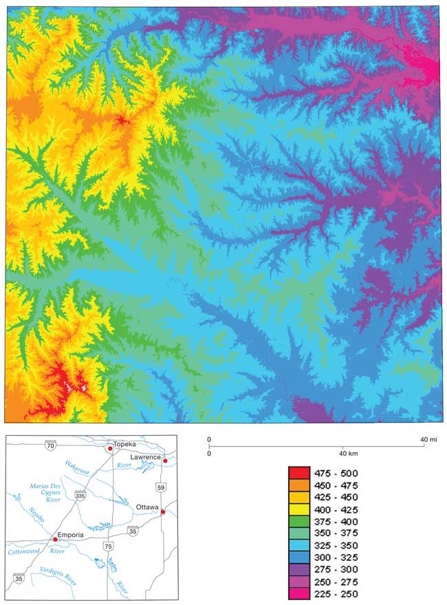
Figure 11 is similar to fig. 10 in that color contours also represent differences in elevation, but there are important differences. In Figure 11, shaded relief has been superimposed over the bands of colors, causing moderate differences in the shades of color, although the same color scheme is used to represent elevations. Most notably in fig. 11, the geographic distribution of the two theoretical gravel layers has been incorporated in the map.
Figure 11--Present topography of experimental area denoted by color contours as in fig. 10, except that hillshading has been superimposed over colors. Additionally, geographic distribution of two theoretical gravel layers has been superimposed (white for upper layer, gray-brown for lower layer). Finally, distribution of actual high-level chert gravels that have been mapped is also superimposed (small patches of red along the current drainage).
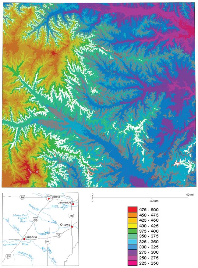
Where the theoretical gravel layers have been "preserved," the colors representing elevations have been suppressed. The upper of the two theoretical gravels is denoted with white, and the lower in brown. Furthermore, when the geographic distribution of the actual chert gravels (fig. 6) is superimposed, the test is the degree to which the theoretical chert gravels and the actual chert gravels coincide as mapped here.
Complete coincidence would be an abstract ideal, and at best in our experiments the degree of coincidence was from far from ideal. If the thickness of either or both theoretical layers was decreased, the theoretical remnants of course were less extensive and would vanish if they were decreased too much. By contrast, if their thicknesses were increased, the remnants would be more extensive, but the degree of coincidence would not necessarily be increased.
After a large number of experiments in which many different combinations of pivot elevations, gradients, thicknesses, intervals, and slope directions were tried, those shown in figs. 8 and 9 were the best that we could determine, based on the degree of coincidence on the map in fig. 11. The parameters of the theoretical chert layers are listed in table 2.
Table 2--Geometrical properties of theoretical chert-gravel layers that best accord with actual high-level chert gravels.
| Direction of slope | S45°E |
| Slope gradient | 0.0002145 (21 cm/km or 14 inches/mi) |
| Thickness of each theoretical layer | 8 m (25 ft) |
| Spacing between theoretical layers | 24.5 m (80 ft) |
| Location of pivot | NW corner experimental area; 39°7'30" N lat, 96°37'30" W long |
The coincidence in fig. 11 is far from perfect, but all things considered it is not bad. The biggest difference is that the geographical extent of the theoretical chert gravels is greater than the actual chert deposits that have been preserved. The correspondence might have been better if actual gravels that correspond to the overall general distribution of the theoretical gravels formerly existed and had been better preserved. Whatever the former areal extent of the actual gravels, much has been removed by erosion in the meantime.
We realize that our assumptions about the two theoretical high-level chert gravels are drastic simplifications. The slopes of the surfaces on which they were deposited ideally should incorporate a gentle exponential decrease toward the southeast. Furthermore, the assumption that each theoretical deposit was 8 m thick exceeds the known maximum thickness of any of the actual remnants of the high-level gravels of about 6 m. Nevertheless, these and other simplifications seem reasonable. Adding assumptions and progressively increasing the trial-and-error modifications would have required more experimentation and likely would not have modified our general interpretations.
Do the parameters as listed provide approximations for the actual ancient chert gravels? If we accept some latitude, they probably do. So if we are reasonably correct, we then are faced with the task of explaining how stream systems in eastern Kansas evolved in which gravels were transported over gradients of little more than 20 cm per km, or a foot per mile.
However, at least one significant exception to the generalized southeasterly gradient exists. Aber (1997, fig. 2) documents a gradient toward the southwest in Anderson County, in the southeastern part of the experimental area, suggesting that there might have been another drainage system entering the region from the north or northwest. We do not have an explanation for this seemingly aberrant drainage direction, unless it was a tributary to one of the ancestral streams that generally drained toward the southeast.
Prev Page--Introduction, Background || Next Page--Fracture System, Lineaments
Kansas Geological Survey
Web version Dec. 26, 2007
http://www.kgs.ku.edu/Current/2007/Harbaugh/03_grad.html
email:webadmin@kgs.ku.edu