Kansas Geological Survey, Petrophysical Series 5
1Kansas Geological Survey
2U.S. Geological Survey
3San Jose State University
Originally published in 1990 as Kansas Geological Survey Petrophysical Series 5. This is, in general, the original text as published. The information has not been updated.
The Simpson Group, a sequence of Middle Ordovician clastic rocks and sandy carbonates, was studied in the subsurface of south-central Kansas. An analysis of lithofacies based primarily on well cuttings permitted the construction of a stratigraphic framework of six informal units. The McLish formation corresponds to the lowermost two of these units and the Bromide formation to the remaining four. Statistical moments of gamma-ray logs were used to characterize the shale content and variability with depth within the Simpson Group. The moments were interpolated between wells and transformed to polynomial trends of estimated shale content in the three dimensions of geographic location and depth. A series of cross sections through this regional three-dimensional model outlines the geometry of major shale and nonshale units. The well cuttings confirm the validity of these patterns and provide more detailed and conventional geologic information for use in their interpretation.
An Acrobat PDF file containing the complete paper is available (3.5 MB).
The Simpson Group in Kansas is a sequence of clastic and sandy carbonate rocks of Middle Ordovician age. Although it contains hydrocarbons, the Simpson Group in Kansas has been neglected in published studies because it lies entirely within the subsurface.
The study area (fig. 1) is in south-central Kansas and consists primarily of Barber, Comanche, Kiowa, and Pratt counties. More specifically, the area includes that part of Kansas located in T. 25-35 S., R. 10-21 W., inclusive. Parts of Clark, Edwards, Ford, Kingman, Reno, and Stafford counties are thus also included. This area has been the focus of a number of studies in the past, both of the Simpson Group (Doveton et al., 1984) and of the Viola Limestone (Bornemann, 1979; St. Clair, 1981; Bornemann et al., 1982; Bornemann and Doveton, 1983). The Pratt anticline, which runs through the center of the area, is an important area of petroleum production in Kansas, and good-quality subsurface data are abundant and readily available.
Figure 1--Location of study area in Kansas.
The Simpson Group was first named by Taff in 1902 from exposures in the Arbuckle Mountains. Most studies of the group have been based on outcrops in southern Oklahoma, especially the Arbuckle Mountains. Ulrich (1911, 1929) named most of the formations. Other important stratigraphic investigations of the Simpson in Oklahoma were conducted by Decker (1930, 1941), Decker and Merritt (1931), Harris (1957), and Statler (1965). Dapples (1955) examined the regional setting of the Simpson Group and its temporal equivalents, especially the St. Peter Sandstone. Schramm (1963, 1964), using both outcrop and subsurface information, conducted a regional study of Simpson lithofacies in Oklahoma.
Because of the lack of outcrops, relatively little has been published on the Simpson Group in Kansas. Ireland (1965) conducted a regional study of the Simpson and correlated the Oklahoma formations into Kansas. Adkison (1972) studied the Simpson Group, the Viola Limestone, and the Sylvan Shale in the Sedgwick basin of south-central Kansas, an area that overlaps the study area in its eastern part.
Witzke (1980) discussed the regional setting of the North American midcontinent during the Middle and Late Ordovician. He showed that the Simpson Group, along with its correlatives, including the St. Peter and Harding sandstones and the Winnipeg Formation, forms a clastic wedge of materials that were shed off the Transcontinental arch (fig. 2). Carbonate rocks were generally more abundant further from the arch.
Figure 2--Simplified Middle Ordovician paleogeography and structural features of the region bordering the Transcontinental arch [modified from Witzke (1980)]. Heavy line corresponds to present Middle Ordovician margin. Boundary between region of dominant clastic and carbonate rocks is generalized.
Witzke's paleogeographic setting thus places the study area at approximately 11° south latitude, in the arid trade winds belt. To the paleonorth (present-day northwest) was the exposed Transcontinental arch, which was the source of clastic material. To the paleosouthwest (present-day south) was the deeper Oklahoma basin. The study area would have been on a shallow marine shelf between the two.
The stratigraphic framework is based primarily on 753 interpreted logs of well cuttings from the Kansas Sample Log Service (fig. 3). Ninety-one of these logs were from outside the study area proper (i.e., from T. 24 S., R. 22-23 W.) but were added to control edge effects on the maps. Most of the logs were interpreted by the same person (J. D. Davies), thus aiding in the consistency of interpretation. The well cuttings data were supplemented by examination of wireline logs, but the latter added little to the results. Thirteen cores from the collection of the Kansas Geological Survey were examined (fig. 4) both megascopically and petrographically (approximately 150 thin sections).
Figure 3--Locations of 753 interpreted logs of well cuttings.
Figure 4--Locations of 13 cores.
The Simpson Group in the study area ranges from 43 to 225 ft (13-69 m) thick. Thickness generally increases toward the south-southeast (fig. 5). Paleogeographic indications show that this would have been a basinward direction.
Figure 5--Isopach map of the total Simpson Group. Contour interval 20 ft.
The upper and lower contacts of the Simpson Group are usually easily distinguishable in the study area. The contact with the underlying dolomites of the Arbuckle Group is a major unconformity between the Sauk and Tippecanoe sequences. Usually a basal sandstone or shale of the Simpson lies with clear contrast on dolomite of the Arbuckle. Occasionally the Simpson lies on a layer of reworked Arbuckle. The upper contact, with the Viola Limestone, is also usually easily discernible because the lowermost Viola in this area is almost always a nonsandy, noncherty, crinoidal limestone. Even where this limestone overlies carbonate rocks of the Simpson, the Simpson carbonates are distinguished by their contrasting sandiness.
Figure 6 is an isopach map of the total thickness of carbonate rock in the Simpson Group in the study area. The abrupt transition from almost no carbonate rock in Barber and Pratt counties to tens of feet of carbonate rock in Comanche and Kiowa counties was initially intriguing. To investigate this transition further, we needed a detailed stratigraphic framework within the Simpson in this area. Based primarily on the 753 sample logs, an informal six-unit stratigraphic framework for the Simpson was constructed. A composite stratigraphic column is shown in fig. 7, but because only one of the units extends over the entire area, any particular location would have fewer than the entire six units.
Figure 6--Isopach map showing total thickness of carbonate rock in the Simpson Group. Contour interval 10 ft.
Figure 7--Composite stratigraphic column of the Simpson Group in the study area showing units A through F.
The lowermost unit within the Simpson Group in the study area is a basal sandstone, which has been designated unit A. As can be seen from the isopach map of this unit (fig. 8), it is thickest [≈60 ft (≈20 m)] in the southern parts of Comanche and Barber counties and thins or is absent to the north. The relatively thin unit A in Pratt County seems to be disconnected from the main body of sandstone to the south and may not be strictly correlative with it. The thinning of unit A near the border of Comanche and Barber counties suggests either some topographic influence of the Pratt anticline at the time of deposition or a slight erosional disconformity between units A and B.
Figure 8--Isopach map of unit A, lower sandstone unit. Contour interval 10 ft.
The lithology, according to the sample logs, is a white to gray fine- to coarse-grained, angular to subrounded, frosted, friable sandstone. It is often phosphatic (sometimes the phosphatic material is replaced by pyrite) and sometimes shaly or dolomitic. Core and thin section examination shows the sandstone to be a poorly sorted quartzarenite with silica or dolomite cement.
The next unit within the Simpson Group in the study area is a sandy green shale, unit B. This is the thickest of all six units and reaches a maximum of 130 ft (40 m) in Barber County. The unit is thickest to the south-southeast and thins toward the northwest to as little as 5 ft (1.5 m) (fig. 9).
Figure 9--Isopach map of unit B, lower sandy shale unit. Contour interval 20 ft.
The sample logs show that unit B is a generally shaly interval with varying amounts of sandstone. The contact with the underlying unit varies from sharp and easily determined to gradational. The sample logs usually describe unit B as an olive-green or green subwaxy, sandy shale with beds of sandstone of the same description as unit A. The sandstones are commonly described as phosphatic. When seen in core, pyrite is often abundant.
Unit C is the second, and main, sandstone within the sequence. This unit is the main hydrocarbon reservoir within the Simpson Group in the study area. This sandstone is thickest in the southeast part of the study area and thins to the northwest (fig. 10). It is a maximum of 90 ft (27 m) thick in southeast Barber County but is absent to the west in parts of Comanche and Kiowa counties.
Figure 10--Isopach map of unit C, upper sandstone unit. Contour interval 20 ft.
The precise contact with the underlying shale of unit B is often difficult to determine. Sandy beds in unit B and shaly beds in unit C can lend uncertainty to which shale-sand transition corresponds to the contact. The lithology is similar to that reported for unit A: a white, gray, or brown fine- to coarse-grained, angular to subrounded, frosted, friable to tight sandstone. Unit C sandstone is much more commonly dolomitic than unit A, especially near the top. Occasionally the top of unit C is reported in the sample logs as a thin zone of sandy dolomite.
Because of its economic importance, unit C is the most commonly cored interval. Core and thin section examinations show the sandstones to be quartzose (fig. 11), but feldspar is commonly present in minor amounts. The quartz grains often have a tattered appearance because of partial replacement by carbonate. Tabular gypsum crystals were found in one sample. Glauconite and pyrite are locally abundant accessories. Phosphatic material is ubiquitous, especially as pellets up to 1 cm (0.4 in.) in diameter. Sorting is usually poor to moderate.
Figure 11--Photomicrograph of quartzarenite from unit C showing quartz overgrowths on many grains. Sample AO4557 from Sinclair-Prairie No. 1 A. Oldfather, sec. 18, T. 31 S., R. 14 W., Barber County, Kansas. The bar scale is 1 mm.
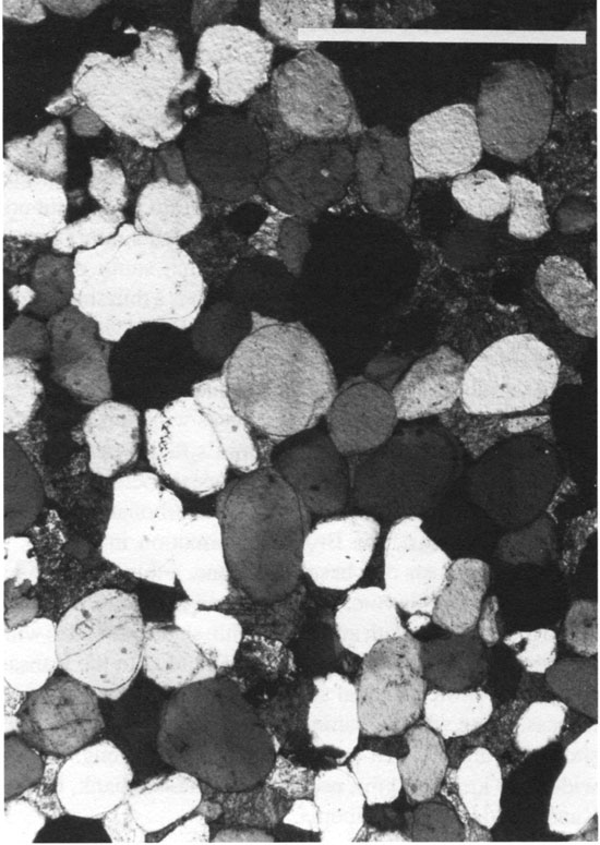
Dolomite and silica cements are most common, but calcite cements also occur. Silica cements are usually in the form of quartz overgrowths (fig. 11). Dolomite cements are commonly zoned, with ferroan layers typically rimming nonferroan layers.
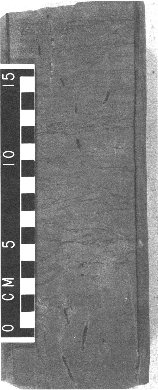
Frequently within unit C a brown sandstone overlies a white sandstone. Stylolites, occasionally filled with shale, are found in some of the cores. Thin, highly contorted layers of green or gray shale are common in the sandstone (fig. 12) but, except for locally abundant Skolithos burrows (fig. 13), few other primary sedimentary structures are evident.
Figure 12--Core showing contorted shale layers in white sandstone in unit C from a depth of 4432 ft (1351 m) in Sinclair-Prairie No. 1 Blurton, sec. 22, T. 28 S., R. 12 W., Pratt County, Kansas.
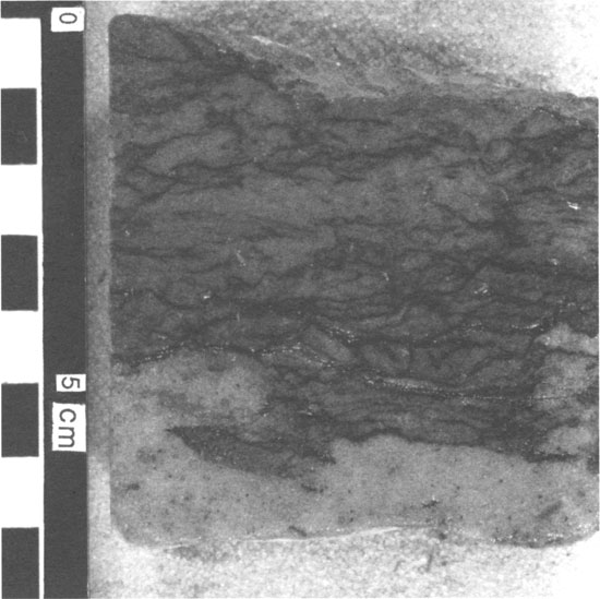
Figure 13--Core showing Skolithos burrows in unit C from a depth of 4243 ft (1293 m) in CRA No. 1 Calbeck "A," sec. 1, T. 27 S., R. 13 W., Pratt County, Kansas.
The pattern of total carbonate thickness, as seen in fig. 6, is controlled primarily by unit D, a sandy, cherty dolomite (fig. 14). This unit is a north-south-oriented carbonate bank or mound with sharp geographic boundaries. The unit is as much as 130 ft (40 m) thick and averages 35 ft (10 m) thick. The eastern edge is particularly sharp, and in places the thickness changes from 0 to 25 ft (0-7.6 m) within a mile.
Figure 14--Isopach map of unit D, sandy, cherty, dolomite unit. Contour interval 20 ft.
The lithology, as described in sample logs, is most commonly a gray-buff to brown cherty, fine to coarsely crystalline, sandy dolomite but the rock also can be a limestone or dolomitic limestone. Unit D is often described as having vuggy porosity. Green shale is occasionally found within unit D, especially toward the north.
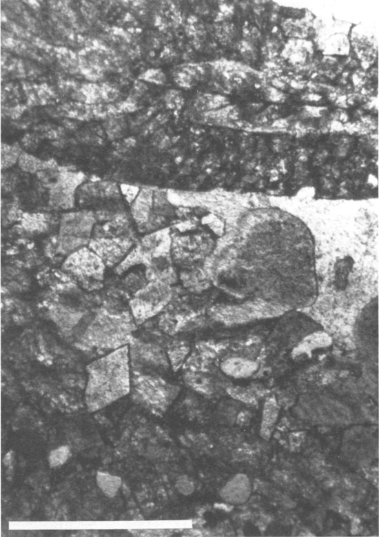
From examination of cores and thin sections, the dolomite commonly occurs in interlocking nonferroan rhombs (fig. 15). As in the sandstones, phosphatic material is a common accessory. The carbonate rocks are the only units with abundant macrofauna (fig. 16). Bryozoans, echinoderms, and ostracodes are common and indicate an environment of normal marine salinities.
Figure 15--Photomicrograph of finely crystalline, nonferroan dolomite from unit D showing interlocking dolomite rhombs. Sample EB6328 from Sinclair-Prairie No. 1 Exchange Bank, sec. 27, T. 33 S., R. 19 W., Comanche County, Kansas. The bar scale is 1 mm.
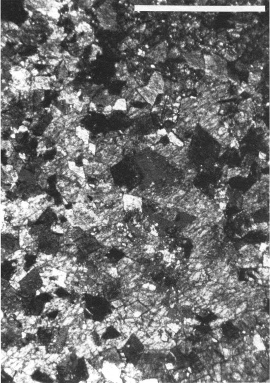
Figure 16--Photomicrocraph of limestone from unit D showing bryozoan and echinoderrn fragments. Sample EB6347 from Sinclair-Prairie No. 1 Exchange Bank, sec. 27, T. 33 S., R. 19 W., Comanche County, Kansas. The bar scale is 1 mm.
Unit E is another green shale, although it is considerably thinner than unit B. It extends over much of the study area (fig. 17) but has a patchy distribution of thick and thin intervals. It can be as much as 50 ft (15 m) thick but averages 12 ft (3.7 m) thick.
Figure 17--Isopach map of unit E, upper shale unit. Contour interval 10 ft.
The lithology is generally described in the sample logs as a green subwaxy, sandy shale. Core examination shows pyrite and phosphatic pellets to be common.
A thin green shale, up to 20 ft (6 m) thick, often lies between units C and D. As unit D is lost to the east, this shale becomes indistinguishable from unit E. It has not been given a separate unit designation but might be a tongue of unit E. The main part of unit E seems to lie above unit D, however.
Unit F is a thin, patchy, sandy limestone. Within the study area it seems to be geographically disjunct from unit D. Unit F represents most of the carbonate rock to the east of the Kiowa-Pratt county border in fig. 6. It is very thin (fig. 18), at most 30 ft (9 m) thick, and usually absent.
Figure 18--Isopach map of unit F, sandy limestone unit. Contour interval 10 ft.
Unit F is easily distinguished from unit D because it is almost never cherty. Unit F is usually a sandy limestone but can be a dolomitic limestone or dolomite. Unit D, in contrast, is usually a dolomite. Sample logs usually describe unit F as a white to gray dense, sandy limestone. No unequivocal unit F was observed in the cores.
Schramm (1963, 1964) studied the regional lithofacies and stratigraphic relations within the Simpson Group in Oklahoma. He constructed maps of the extent of each of the six formations comprising the Simpson and showed facies variations within each. From oldest to youngest these are the Joins, Oil Creek, McLish, Tulip Creek, Bromide, and Corbin Ranch formations. Three of these formations (the Joins, Tulip Creek, and Corbin Ranch) are limited to southern Oklahoma. One, the Oil Creek, terminates close to the Kansas-Oklahoma border. The other two formations, the McLish and the Bromide, extend into Kansas.
A tentative correlation of units A through F with the formation names used in Oklahoma is presented in fig. 19. Key to this correlation is a columnar section of the Sinclair Oil Co. No. 1 Berry well given by Schramm (1963) but not reproduced in Schramm's 1964 article. In Schramm's section, located in Ellis County, Oklahoma, south of Clark County, Kansas, the Oil Creek Formation is a thin shale. This formation disappears between the No. 1 Berry well and the Kansas border. The McLish Formation in that well consists of a basal sandstone, a medial shale, and an upper dolomite. The basal sandstone probably correlates with unit A and the shale with unit B. Because Schramm's facies maps of the McLish show that the carbonate disappears before reaching the Kansas border, there is no correlative carbonate unit in the McLish in Kansas. The Bromide Formation in the No. 1 Berry well consists of a basal sandstone, a thin shale, and a thick overlying dolomite. The sandstone correlates with unit C and the dolomite with unit D. The thin shale correlates with the thin shale often separating units C and D in the Kansas study area. More regional studies of the Simpson Group in Kansas, along with Schramm's facies maps of the Bromide, show that unit D is an approximately 150-mi-long, 50-mi-wide (240 km x 80 km), north-south-oriented bank, half in Kansas and half in Oklahoma.
Figure 19--Correlation of units A through F with McLish and Bromide formations of Oklahoma. Sinclair No. 1 Berry (Ellis County, Oklahoma) interpretation from Schramm (1963).
The Simpson Group in the study area consists of clastic and carbonate rocks deposited on a shallow marine shelf. Evidence for this conclusion comes primarily from paleontologic and paleogeographic considerations. The depositional environments of extensive blanket sands before development of land plants are a subject of controversy. There has been some success in modeling the environments in areas with good outcrops (Dott et al., 1986), but the sparseness of core data and diagnostic sedimentary structures in this study require that the environmental interpretation not be based primarily on lithology.
Macrofossils are uncommon, except in the carbonate rocks, but the fauna includes such stenohaline organisms as echinoderms, bryozoans, and brachiopods. Microfaunas have also been collected from the Simpson Group in this area and include conodonts, which are also stenohaline. Skolithos burrows in unit C are suggestive of shallow marine environments.
Fragmental plates of fossil fish also have been recovered from the sandstones. Fossil fish debris is not uncommon in the Ordovician of the midcontinent, where it is sometimes recovered as a by-product of the search for conodonts. The best-known occurrence of Middle Ordovician fish in the area is from the Harding Sandstone of Colorado (Denison, 1967; Spjeldnaes, 1979). There is some debate over whether early fish lived in salt- or freshwater. The associated fauna in the Simpson clearly indicates normal marine salinities, but the fragmentary nature and roundness of the fish plates does not rule out transportation from a freshwater source.
Deposition of the McLish formation within the study area can be modeled by a transgressive sequence of a higher-energy nearshore sandstone unit (unit A) and a lower-energy offshore shale unit (unit B) (fig. 20). Units C and E within the Bromide formation are analogous to units A and B in the McLish formation. The lithologic similarities suggest that they also represent a transgressive sequence with unit C as the higher-energy nearshore sandstone and unit E as the lower-energy offshore shale.
Figure 20--North-south cross section (line D-D' in figs. 23-25) of the McLish Formation. The datum is the top of unit B.

The carbonate bank that makes up unit D overlies the northwesternmost edge of the unit C sandstone (fig. 21). If unit C is transgressive from southeast to northwest, the northwestemmost edge would be the youngest part of unit C. This would make unit D younger than unit C, at least in the study area. If the thin green shale that sometimes lies between units C and D actually correlates with shale unit E, then one of two possible event sequences took place: The carbonate bank of unit D was deposited contemporaneously with basinward shales that form part of unit E, or the time of deposition of unit D is represented in the eastern part of the study area by a diastem.
Figure 21--East-west cross section (line R-R' in figs. 23-25) of the Bromide Formation. The datum is the top of the Simpson Group.
Unfortunately, the other carbonate unit, unit F, is not represented with certainty in any of the cores. Stratigraphic position and general lithologic descriptions from the sample logs do not provide sufficient information to determine depositional environment.
The proposed correlation with Oklahoma formations and the proposed event sequence suggest an unconformity above unit B. Especially in the eastern part of the study area, this contact is often difficult to identify and in some sample and well logs could be interpreted as gradational. None of the examined cores preserve the actual B-C contact. We believe, however, that, in the absence of solid evidence for a gradational contact, the unconformity is genuine.
The proposed chronology of depositional events, therefore, begins with nearshore sandstones (unit A) and offshore shales (unit B) being deposited contemporaneously as a transgressive sequence from south to north. Regression led to an unconformity above this sequence. A similar nearshore sandstone (unit C) and offshore shale (unit E) were then deposited as a transgressive sequence from southeast to northwest. After unit C was deposited, a carbonate bank (unit D) was established in a nearshore position while shales of unit E continued to be deposited offshore. Final events in the deposition of the Simpson Group in this area, including the deposition of carbonate unit F, are not clear.
The isopach maps of the Simpson Group units (figs. 8-10, 14, 17, 18) show distinctive regional patterns of distribution that reflect depositional environment. The simultaneous consideration of all six maps is difficult, even when aided by the production of a single composite lithofacies map, because compositional changes occur in the three dimensions of depth and geographic space and any map or section is restricted to the two dimensions of the paper. This limitation has been recognized for many years, and various methods to provide maps that give information on vertical variation have been suggested.
Krumbein and Libby (1957) reviewed these "vertical variability maps," which range from maps of simple statistics, such as number of sandstone beds, to maps showing ratios of sand compositions between unit subdivisions, and introduced a new approach to the problem. They expressed vertical variation in the form of moments of the vertical distribution and then mapped these moments. This methodology has important advantages. Moments are fundamental measures of variability, which have simple meanings in both statistics and mechanics. Moments are easy to compute and are an improvement over earlier pragmatic methods. Although there is a succession of higher moments, Krumbein and Libby (1957) restricted their consideration to the first two moments. These correspond to the center of gravity and the radius of gyration of the distribution of lithology. Maps of these two moments, used in conjunction with conventional facies maps, give basic insight into gross compositional changes in three dimensions.
We extended the moments method to the direct expression of lithofacies variation as a function of both geographic location and depth. This is possible because the coefficients of polynomial regression curves are defined uniquely by moments. These curves can be used to define trends of variation across three spatial dimensions. The analytical data were drawn from all available gamma-ray logs in the study area to provide a simple but effective measure of shale content at each well location. The aim of this new technique was to produce three-dimensional images of large-scale shale features and (their complement) sandstone and carbonate bodies. The abundance of well cuttings descriptions were valuable as "ground truth" to validate the results and discriminate real facies geometry from mathematical artifacts. The stratigraphy of unit subdivisions, defined earlier, provided the reference framework for correlation and a key to the interpretation of the genesis of observed trends and features in the three-dimensional model.
The gamma-ray log from Sohio Swisher No. 1, C SW NW sec. 2, T. 29 S., R. 13 W., in Pratt County is shown in fig. 22 and is a typical example of the Simpson Group in the eastern part of the study area. In the local driller's informal terminology, the section shows the "Simpson sand" overlying the "Simpson shale." If we apply the stratigraphic framework proposed here, the sequence consists of unit B (shale), unit C (sandstone), and unit E (shale). The well was a wildcat well that resulted in an oil discovery in the Simpson Group.
Figure 22--Gamma-ray log of the Simpson Group from Sohio Swisher No. 1, C SW NW sec. 2, T. 29 S., R. 13 W., Pratt County, Kansas.
The gamma-ray log allows a simple distinction to be made between radioactive shales and less radioactive sandstones and carbonates. The sources of radioactivity in shales are primarily thorium, adsorbed on clay minerals, and potassium-40, which is a constituent of some clay minerals. Uranium is sometimes an important contributor but is mostly associated with "black shales," in which reducing conditions and high organic content result in extensive fixation of reduced uranyl ion and consequent anomalously "hot" gamma-ray values. By contrast, typical sandstones and carbonates register relatively low levels of radioactivity, which usually reflects minor contents of clay minerals, micas, and feldspars. Because the gamma-ray response is a function of the weight concentration of radioactive isotopes, the log can be used to estimate volumetric proportion of shale at any given depth. The range in gamma-ray readings from a typical shale baseline to a sandstone (or carbonate) baseline is proportionally scaled (fig. 22). The result is a simple transformation of the log into a "shale profile" of the stratigraphic section, expressed as shale content rather than in arbitrary count units.
The rescaled log expresses the vertical variation in shale content, which must be condensed in some manner to be mapped. The most basic measure is the average amount of shale, or the mean shale reading. If the log is digitized, conventionally at two readings per foot, the mean proportion of shale in the section is
where n is the number of readings and Si is the proportion of shale at depth i. The center of gravity of the vertical distribution of shale can then be computed from the equation
![]()
where d is the depth of the ith value. Depths are measured from the top of the stratigraphic unit. The center of gravity is the first moment and locates the balance point of the shale distribution on the depth axis.
The second moment of shale variation is given by
![]()
which statistically expresses the relative amount of dispersion of the shale distribution with depth from the top of the unit. Generally, the second moment is modified so that it expresses dispersion about the center of gravity:
![]()
The quantity m2 is called the relative standard deviation, and it corresponds to the radius of gyration of the distribution when rotated about the center of gravity.
A progressive series of moments can be calculated from the general formula
![]()
where Vm is the mth moment. The third moment is a measure of skewness, which expresses the direction and degree of asymmetry of a distribution. The fourth moment expresses kurtosis, or the relative peakedness of the shape of a distribution. Higher moments express more subtle aspects of distribution shape, require the calculation of large numbers, and may become unstable because of rounding.
In the form presented here the moments are expressed in terms of depth (measured in feet or meters). This means that the moments are sensitive to the total thickness of the unit over which they are calculated. The difference between moments from two wells may indicate different vertical distributions of shale or simply that the total interval is thicker in one well. To avoid this ambiguity, we express the moments in proportional form, achieved by dividing the moment by the total thickness. Because of the division, the units of depth cancel and the proportional moment is unitless.
The reference log (fig. 22) shows the top and the base of the Simpson Group, its mean shale composition, and the center of gravity and standard deviation of the shale distribution. These descriptors were calculated for gamma-ray logs from 148 wells in the study area. The mean shale ratio map (fig. 23) contains three broad belts arranged in a general north-south orientation. Regions characterized by relatively low shale (high sand) proportions to the east and west are broken by a high- shale trend centered over the Pratt anticline. A map of the proportional centers of gravity (fig. 24) contains relatively high values that indicate that the bulk of the shale is in the lower part of the Simpson Group. Conversely, the bulk of the sand must be in the upper part. The proportional standard deviation map (fig. 25) indicates that shale intervals are more highly dispersed throughout the section in those locations where the proportion of shale in the Simpson is highest.
Figure 23--Mean shale ratio map of the Simpson Group. Ratios higher than 0.5 are shaded. Lines D-D'and R-R' locate cross sections used in figs. 20, 21, 28, 30, 3 1, and 32.
Figure 24--Center of gravity map of shale distribution in the Simpson Group. Values higher than 0.5 are shaded. Lines D-D'and R-R' locate cross sections used in figs. 20, 21, 28, 30, 31, and 32.
Figure 25--Relative standard deviation map of shale distribution in the Simpson Group. Values higher than 0.25 are shaded. Lines D-D' and R-R' locate cross sections used in figs. 20, 21, 28, 30, 31, and 32.
The isopach map and the three shale moment maps must be compared in detail, possibly by overlaying them in sets, to be interpreted. The process involves collating several two-dimensional summaries of variation in the vertical dimension to arrive at a three-dimensional visualization of the distribution of sand and shale. However, the moments are statistics whose values specify unique shapes of vertical variation. A set of moment maps defines three-dimensional variation precisely and quantitatively. Therefore the qualitative interpretation of moment maps is only an intermediate step in the quantitative generation of a three-dimensional model of lithologic variation.
The shale profile in fig. 22 was analyzed by fitting a polynomial regression to the measurements of shale composition. A first-order polynomial is a straight line defined by the equation
![]()
where ![]() is the estimated proportion of shale at depth d, as predicted by a line with intercept a0 and slope a1. The unknown coefficients are found by solving the simple matrix equation
is the estimated proportion of shale at depth d, as predicted by a line with intercept a0 and slope a1. The unknown coefficients are found by solving the simple matrix equation
The first-order polynomial fitted to the measurements of shale in the reference section is shown in fig. 26. The line defines a trend of increasing shale content with depth.
Figure 26--Zeroth- through fourth-order polynomial regression trends of the reference gamma-ray log shale profile (fig. 22).
A quadratic (or second-order) polynomial function describes a curve with a single maximum or minimum. It can be fitted to the shale profile by the equation
![]()
The matrix equation that provides the three unknown coefficients is
All information about the proportion of shale in the section is contained in the vector on the right-hand side of Eqs. (7) and (9). All terms on the left-hand side involve either the number of observations or the depths to the measurement points and do not consider the proportions of shale at all. If the righthand vector is divided by the sum of the proportions of shale, ΣS, then the first term will become ΣS/ΣS = 1.0. The next two terms will be, respectively, ΣSd/ΣS and ΣSd2/ΣS, which are the first two moments of the vertical distribution of shale. From this it can be seen that the moments define a polynomial function. In this instance the mean shale content, center of gravity, and standard deviation collectively define a unique polynomial curve of the proportion of shale as a function of depth. In a similar fashion the matrix equation used to fit a first-order polynomial is based on the mean shale content and the center of gravity or first moment of the shale distribution. An even simpler zeroth-order polynomial can be defined by the equation

The coefficient is equal to the average proportion of shale within the stratigraphic section.
More complicated curves can be fitted to the vertical distribution of the proportion of shale by expanding the size of the polynomial functions. For each additional coefficient the matrix equation must be expanded by one row and one column. The general form of the matrix equation is
and is uniquely determined by the mean and first m moments.
An interesting corollary is that, if polynomial curves are defined by the moments of the distribution, then the vertical variability that can be interpreted from a set of moment maps is predetermined. From a combination of a mean shale content and a center of gravity map, only a linear trend can be inferred at any location. The addition of a standard deviation map allows variation to be expressed as either a maximum or a minimum within the section but precludes the expression of more complex patterns of vertical variation.
The relationship between moments and polynomial curves can be used to predict the number of moment maps that are necessary to characterize the vertical variability of a stratigraphic unit. The goodness of fit of a polynomial curve to the vertical distribution of shale in a section can be found as a percentage of the total variation in shale content. Higher-order polynomials will define increasingly more complex curves that progressively fit the section more closely until the pattern of variation is matched perfectly. This is demonstrated in fig. 27, in which polynomial equations are fitted to the reference log; the higher-order curves more faithfully represent the vertical variation in shale content.
Figure 27--Percentage fits of polynomial regression orders to reference gamma-ray log shale profile (fig. 22).
In a plot of the fit of the polynomial curves against the order of the polynomials, it is sometimes possible to identify an equation that represents a systematic major trend. Such a graph for the reference log (fig. 27) indicates that a third-order polynomial is an appropriate choice to represent the major pattern of shale variation in the section. This implies that the Simpson Group is composed of two major subdivisions that correspond to the two extrema allowed by the cubic equation. This mathematical conclusion matches the visual evidence of the gamma-ray log (fig. 22), in which the two subdivisions can be identified with units B and C. The greater thickness of these two units relative to unit E is the reason why they dominate the major trend in the polynomial.
Contour maps that represent the lateral variation in the moments computed from logs at control wells can be made. The reliability of such maps depends to a large degree on the density of well control. The lower moments indicate major shifts in the distribution of shale content, and it is likely that they can be mapped with nearly the same degree of confidence as thickness or structure. This is an implicit assumption in the method of moment mapping pioneered by Krumbein and Libby (1957).
In mapping it is necessary to estimate the moments by interpolation at all locations except at the control wells. These interpolated estimates of moments can be inserted into the matrix equation for a polynomial curve. Then the solved coefficients define a curve of vertical variability that is projected from wells in the immediate vicinity. This can be expressed as a matrix equation,
DA = S, (12)
the solution of which is
A = D-1S, (13)
where D is a depth matrix whose elements are sums of powers of the depth increments in the digitized record, D-1 is the inverse of this matrix, A is the trend coefficient vector, and S is the moment vector, which contains the estimated moments.
Values in the depth matrix depend on the thickness of the section, either measured at a well or interpolated between wells. However, there is a great computational advantage to standardizing all interpolated sections to a constant thickness equal to 1.0: The depth matrix will be a constant regardless of location, so the matrix must be inverted only once in any application. In addition, this limits the magnitudes of the depth measurements, avoiding the possible creation of an ill-conditioned matrix and consequent problems with round-off errors. The polynomial coefficients are scaled to the fixed arbitrary depth but can be transformed easily to true depth measurements by rescaling to the correct thickness.
In summary, the coefficients of a polynomial curve can be estimated at any location in an area by a matrix operation performed on moments interpolated from well control. When these coefficients are combined with estimated thicknesses taken at any location from an isopach map, a polynomial curve that represents the vertical variability in lithology can be created.
The major obstacle to the use of this method is the difficulty of displaying variation in three dimensions on a two-dimensional medium, such as paper or a computer terminal screen. One solution is to map vertical variation as a series of two-dimensional slices and combine these to give the framework of a three-dimensional model. To illustrate the procedure, we calculated an east-west cross section through the Simpson Group (line R-R' in figs. 23-25) and generated a series of cross sections to demonstrate the effect of the different moments on the pattern of regional shale variation (fig. 28). Each section is defined by a grid whose columns correspond in width to a geographic cell and whose rows represent 10-ft (3.0-m) increments of depth. Each column corresponds to a unique geographic position along the cross section. After interpolating the moments from adjacent control wells, we solved for the polynomial trend coefficients at the location corresponding to each column. We then found the estimated proportion of shale at each 10-ft (3.0-m) increment of depth by evaluating the polynomial equations. The resulting grid of shale values was contoured in the same manner as a conventional map. We repeated the procedure using progressively more moments to produce the cross sections shown in fig. 28.
Figure 28--Zeroth- through fourth-order proportion of shale trend profiles of an east-west cross section (line R-R' in figs. 23-25).
The simplest cross section is the zeroth-order one, which is determined solely by the mean shale content at any location. The profile consists of vertical contours of shale proportion because each column consists of a constant value and because no vertical variability can be perceived. The first-order profile is generated from interpolated values of the mean shale content and the center of gravity. These specify a linear trend so that at any location the proportion of shale in the column changes at a uniform rate from top to bottom. The higher-order profiles incorporate successively the second, third, and fourth moments. These markedly improve the resolution of the distinctive shapes and gradations that reflect vertical and lateral facies changes within the Simpson Group. Note that there are relatively minor differences between profiles of the third and fourth order. The cubic polynomial appears to represent the major trend in proportion of shale over much of the region, as was the case with the gamma-ray log example (figs. 26 and 27) discussed earlier. This character reflects the domination of the Simpson Group by units B and C in the east and by units B and D in the west. Statistical analyses of the reference log indicates that the third- and fourth-order profiles express approximately 50% of the total variation in the proportion of shale--if the reference log is typical of the Simpson as a whole. The remaining variation is compounded from small-scale features, many of which persist only locally.
Polynomial functions have other simple properties that provide useful parameters for mapping. If a polynomial equation of the form
![]()
is differentiated, the result is
![]()
which gives the slope of the polynomial curve at any depth. The locations of the peaks and troughs of the curve can be found by setting the slope equation to zero and solving for depth. The cubic polynomial fitted to the reference log yields a quadratic slope equation with two depth values as solutions. The depths correspond to the trend estimate of the maximum and minimum shale development within the section (fig. 29).
Figure 29--Reference gamma-ray log shale profile and fitted cubic trend indexed with maximum, minimum, and inflection-point depths.
If the slope equation is differentiated, the result expresses the rate of change in slope:
![]()
The rate of change is zero at the inflection points of the curve; these mark the boundaries between the maximum and the minimum developments of the shale. On the reference log there is a single solution for the depth of the inflection point (fig. 29). This locates an estimate of the contact between the lower shale subdivision (unit B) and the upper sandstone unit (unit C) based on the cubic polynomial fit to the shale distribution.
The inflection points can be traced across the profiles because their determination depends only on the polynomial coefficients and section thickness of each column. Inflection points on successive grid columns can be linked to sketch boundaries of the lithologic subdivisions. The result is a mathematical interpretation of the lithostratigraphy based on the differentiation of major trends in vertical variability.
The cross section created from fourth-order profiles can be used to illustrate the application of this method. A fourth-order polynomial has two possible inflection points; these were found for all columns along the profile. Only one of the inflection points can be traced as a laterally continuous boundary across the Simpson Group section (fig. 30). At some locations the second solution is irrational, and at other locations the additional inflection point picks out the local development of the basal sand facies (unit A) or the upper shale facies (unit E).
Figure 30--Gamma-ray logs of Simpson Group with simplified fourth-order trend shale ratio profile of east-west cross section (line RR' in figs. 23-25). Internal solid curves trace inflection-point boundaries within the Simpson Group.
Because the slice is derived entirely from a mathematical treatment of gamma-ray logs, which are sensitive only to shale variation, additional geologic information is required for detailed interpretation. Information from representative well cuttings from nearby wells was used to generate a lithologic cross section for comparison with the gamma-ray slice (fig. 31). The basal sandstone (unit A) appears as a localized tongue in the west and is overlain by the thick shale of unit B across the area. The large low-shale-content feature in the west consists of sandy dolomites and limestones (unit D) that are locally underlain by dolomitic sandstones of unit C. The abrupt eastern boundary of this carbonate body coincides with the western edge of the Pratt anticline. The low -shale -content anomalies in the eastern part of the cross section represent sandstone bodies (unit C) that are capped locally by thin sandy dolomites and overlain by shale (unit E).
Figure 31--East-west lithologic cross section based on well cuttings in the neighborhood of line R-R'. The datum is the top of the Simpson Group.
A second gamma-ray slice and lithologic cross section is shown in fig. 32 for a north-south line (line D-D' in figs. 23-25) oriented perpendicular to the regional depositional strike. This profile was also generated from a fourth-order polynomial solution. Again, only one regionally continuous inflection point can be traced through the Simpson Group, although a second inflection point indicates local facies units. The most pronounced secondary facies consists of the basal sandstone unit A occurring at the south end of the section. Low-shale-content features in the upper unit (Bromide formation) are sandstone bodies of unit C, which contain small, localized oil fields, generally with thin pay zones near the top of the sandstone.
Figure 32--Fourth-order proportion of shale trend profile of a north-south cross section (line D-Din figs. 23-25) of the Simpson Group (above) and lithology section based on well cuttings (below).
Three-dimensional gamma-ray shale profiles were computed and mapped along 10 east-west and north-south lines. The locations of these profiles are shown with reference to the mean shale ratio map (fig. 33). The five east-west profiles (fig. 34) and five north-south profiles (fig. 35) allow the visualization of trends in the geometry of major lithofacies across the area. A fence diagram of lithology cross sections (fig. 36) is drawn from the logs of well cuttings and provides a compositional key to the nonshale features. Most important for this experimental application, the lithology cross sections substantiate the patterns generated by the moment method. The technique is therefore a useful geologic tool and would be particularly valuable in applications for which conventional geologic data from cores and well cuttings are sparse.
Figure 33-Location lines of profiles shown in figs. 34 and 35 on mean shale ratio map.
Figure 34-Fourth-order proportion of shale trend profiles of east-west sections (locations shown in fig. 33).
Figure 35-Fourth-order proportion of shale trend profiles of north-south sections (locations shown in fig. 33).
Figure 36-Fence diagram of lithology cross sections based on well cuttings (locations shown in fig. 33).
The transformation of moment maps to three-dimensional representations is not confined to the generation of cross sections. Horizontal slices that portray trend estimates of the shale proportion at any specified depth can be produced. The trend projection of the proportion of shale at the top of the Simpson Group is particularly easy to compute because this level corresponds to a depth of zero. If a value of d=O is inserted into any polynomial, such as
![]()
![]()
The shale content at the base of the Simpson Group can be estimated in an equally straightforward manner. The algorithm solution of the polynomial coefficients uses a standardized depth scale in which the thicknesses of all Simpson Group sections are fixed at 1.0. On this transformed scale the depth of the base of the Simpson Group is 1, and the solution for the shale content is therefore
The proportions of shale in the basal part of the Simpson Group were mapped by estimating the polynomial coefficients over a gridded areal network and contouring their sum (fig. 37). This map is particularly interesting because it defines the lateral extent of the basal transgressive sand (unit A). The pattern of distribution of unit A shows good concordance with the isopach map (fig. 8) of this unit based on drill cuttings.
Figure 37-Fourth-order proportion of shale trend at base of Simpson Group. Proportions greater than 0.3 are shaded, and those greater than 0.7 are heavily shaded.
It is possible to compute other trend maps of shale content either by proportional levels within the Simpson Group or at absolute depths given in feet or meters. In fact, it is possible to compute the shale variation throughout the entire three-dimensional extent of the Simpson Group wedge. This would create a three-dimensional cell structure in which each cell is defined by its geographic coordinates and depth and an associated estimate of the proportion of shale. The essential problem is in displaying such a three-dimensional model in an efficient and effective manner.
The Simpson Group in south-central Kansas can be divided into six informal lithofacies units. The lowermost two units, a basal sandstone and a green sandy shale, correspond to the McLish Formation of Oklahoma. The other four units, a sandstone, a cherty, sandy dolomite, a green shale, and a sandy limestone, correspond to the Bromide Formation of Oklahoma. The cherty, sandy dolomite seems to be part of a carbonate bank with sharp boundaries.
The depositional history of the Simpson Group in this area began with a transgression from south to north and deposition of a clastic sequence consisting of a nearshore sand (unit A) and an offshore shale (unit B). A regression created an unconformity that was subsequently covered by another transgressive sequence of nearshore sand (unit C) and offshore shale (unit E). After deposition of the sand but while the shale was still being deposited offshore, a large carbonate bank was deposited in the western part of the study area. Later events in the chronology, including deposition of a thin carbonate unit (unit F) in the eastern part of the area, are unclear.
The interpolation of statistical moments of gamma-ray logs between well controls was used to generate computer maps of shale trends in three dimensions. These profiles allow direct visualization of the shapes and dispositions of major lithofacies across the study area. Geologic descriptions from numerous drill-cutting records validate the patterns shown by this experimental technique and provide additional distinctions between sandstone and carbonate facies.
Adkison, W. L., 1972, Stratigraphy and structure of Middle and Upper Ordovician rocks in the Sedgwick basin and adjacent areas, south-central Kansas: U.S. Geological Survey, Professional Paper 702, 33 p. [available online]
Bornemann, E., 1979, Well log analysis as a tool for lithofacies determination in the Viola Limestone (Ordovician) of south-central Kansas: Ph.D. dissertation, Syracuse University, Syracuse, New York, 151 p.
Bornemann, E., and Doveton, J. H., 1983, Lithofacies mapping of Viola Limestone in south-central Kansas, based on wireline logs: American Association of Petroleum Geologists, Bulletin, v.67, no.4, p. 609-623
Bornemann, E., Doveton, J. H., and St. Clair, P. N., 1982, Lithofacies analysis of the Viola Limestone in south-central Kansas: Kansas Geological Survey, Petrophysical Series 3, 44 p.
Dapples, E. C., 1955, General lithofacies relationship of St. Peter Sandstone and Simpson Group: American Association of Petroleum Geologists, Bulletin, v. 39, no. 4, p. 444-467
Decker, C. E., 1930, Simpson Group of Arbuckle and Wichita Mountains, Oklahoma: American Association of Petroleum Geologists, Bulletin, v. 14, no. 12, p. 1493-1505
Decker, C. E., 1941, Simpson Group of Arbuckle and Wichita Mountains of Oklahoma: American Association of Petroleum Geologists, Bulletin, v. 25, no. 4, p. 650-667
Decker, C. E., and Merritt, C. A., 1931, The stratigraphy and physical characteristics of the Simpson Group: Oklahoma Geological Survey, Bulletin 55, 112 p.
Denison, R. H., 1967, Ordovician vertebrates from western United States: Fieldiana, Geology, v. 16, no. 6, p. 131-192
Dott, R. H., Jr., Byers, C. W., Fielder, G. W., Stenzel, S. R., and Winfree, K. E., 1986, Aeolian to marine transition in Cambro-Ordovician cratonic sheet sandstones of the northern Mississippi Valley, U.S.A.: Sedimentology, v. 33, no. 3, p. 345-367
Doveton, J. H., Zhu, K.-A., and Davis, J. C., 1984, Three-dimensional trend mapping using gamma-ray well logs-Simpson Group, south-central Kansas: American Association of Petroleum Geologists, Bulletin, v. 68, no. 6, p. 690-703
Harris, R. W., 1957, Ostracoda of the Simpson Group of Oklahoma: Oklahoma Geological Survey, Bulletin 75, 333 p.
Ireland, H. A., 1965, Regional depositional basin and correlations of Simpson Group: Tulsa Geological Society Digest, v. 33, p. 7489
Krumbein, W. C., and Libby, W. G., 1957, Application of moments to vertical variability maps of stratigraphic units: American Association of Petroleum Geologists, Bulletin, v. 41, no. 2, p. 197-211
St. Clair, P. N., 1981, Depositional history and diagenesis of the Viola Limestone in south-central Kansas: M.S. thesis, University of Kansas, Lawrence, 66 p.
Schramm, M. W., Jr., 1963, Paleogeologic and quantitative lithofacies analysis of the Simpson Group, Oklahoma: Ph.D. dissertation, University of Oklahoma, Norman, 84 p.
Schramm, M. W., Jr., 1964, Paleogeologic and quantitative lithofacies analysis, Simpson Group, Oklahoma: American Association of Petroleum Geologists, Bulletin, v. 48, no. 7, p. 1164-1195
Spjeldnaes, N., 1979, The palaeoecology of the Ordovician Harding Sandstone (Colorado, U.S.A.): Palaeogeography, Palaeoclimatology, Palaeoecology, v. 26, nos. 3-4, p. 317-347
Statler, A. T., 1965, Stratigraphy of the Simpson Group in Oklahoma: Tulsa Geological Society Digest, v. 33, p. 162-211
Taff, J. A., Atoka folio, Indian territory: U.S. Geological Survey, Geologic Atlas Folio Series 79
Ulrich, E. O., 1911, Revision of the Paleozoic systems: Geological Society of America, Bulletin, v. 22, p. 281-680
Ulrich, E. O., 1929, New classification of the Paleozoic deposits in Oklahoma: Geological Society of America, Bulletin, v. 40, no. 1, p. 85-86
Witzke, B. J., 1980, Middle and Upper Ordovician paleogeography of the region bordering the Transcontinental arch; in, Paleozoic Paleogeography of the West-Central United States, T. D. Fouch and E. R. Magathan, (eds.): Society of Economic Paleontologists and Mineralogists, Rocky Mountain Paleogeography Symposium 1, p. 1-18
Kansas Geological Survey
Comments to webadmin@kgs.ku.edu
Web version updated April 7, 2010. Original publication date 1990.
URL=http://www.kgs.ku.edu/Publications/Bulletins/PS5/index.html