Kansas Geological Survey, Ground Water Series 3, originally published in 1980
Next Page--Appendices with Source Code
Water is a valuable resource of the State of Kansas. Much money and effort are expended each year to collect various kinds of data. The data base is massive and still is not complete. It is clear that computer storage and manipulation are necessary to make full use of the data. Many pumping tests have been made through the years to help determine the aquifer transmissivity and storage coefficient (transmissivity is a measure of how easily water flows through the earth; and the storage coefficient is a measure of how much water is stored per unit volume). Undoubtedly, many more pumping tests will be made in the future.
Some means of automating the analysis of these pumping tests would be desirable. That is the goal of this work. The method is simple, quick, and inexpensive. However, access to a computer capable of using the FORTRAN language is necessary. The automated analysis has the advantage that it is always objective and cannot consider any personal bias. The method also gives an indication of how well it could analyze the data. The method is not universally applicable to all pumping tests, but has been designed to analyze data conforming to assumptions implicit in the Theis equation.
Through the years, the Theis equation has played an important role in groundwater hydrology. Comparison of experimental pumptest data with this theoretical curve by graphical means has been a standard method of determining aquifer transmissivity and storage. The purpose of this paper is to present techniques and computer programs to evaluate the Theis equation, to evaluate the sensitivity with respect to transmissivity and storage, and to automatically fit experimental pumptest data to the Theis equation obtaining the "best" transmissivity and storage in the least squares sense. The automated fit for pumptest data developed in this work should be a useful tool for the groundwater hydrologist. It is simple to use, quick and inexpensive. The automated fit has the advantage that it is always objective. As a measure of the error in fitting, the rms error in drawdown is calculated for the "best" transmissivity and storage.
Through the years, the Theis equation has played an important role in groundwater hydrology (Theis, 1935). Comparison of experimental pumptest data with this theoretical curve by graphical means has been a standard method of determining aquifer transmissivity and storage (Jacob, 1940). The purpose of this paper is to present techniques and computer programs to evaluate the Theis equation; to evaluate the sensitivity with respect to transmissivity and storage; and to automatically fit experimental pumptest data to the Theis equation, obtaining the "best" transmissivity and storage in the least squares sense. For a more detailed discussion of sensitivity coefficients and their uses, see McElwee and Yukler (1973).
The Theis equation involves an integral whose upper limit is infinity. Evaluation of this integral is considered in the section on numerical approximation. After the Theis equation has been evaluated, the sensitivity coefficients can be obtained with little additional work. These sensitivity coefficients are used in the section on least squares fitting to develop an algorithm for fitting the Theis equation to experimental pumptest data. The automated method is simply, quick, and inexpensive. The automated method has the advantage of always being objective and always indicating its error by calculating the rms error in drawdown.
The Theis equation (Theis, 1935) describes radial confined groundwater flow in a uniformly thick horizontal, homogeneous, isotropic aquifer of infinite areal extent.
S = (Q / 4πT) ∫(r2s/4Tt)∞ [(e-u/u) du] (1)
The radius of the pumped well is assumed negligible (line source or sink approximation). The derivation and solution is documented many places (Jacob, 1940) and will not be discussed further here. In the above equation s is drawdown (L), Q is the discharge (L3/T), T is the transmissivity (L2/T), t is the time (T), S is the dimensionless storage coefficient, and r is the radial observation distance from the pumped well (L). L and T in the preceding parentheses are arbitrary units of length and time.
Usually, the Theis equation is fitted graphically to experimental pumptest data to obtain approximations for the storage coefficient (S) and the transmissivity (T). In this paper an algorithm will be presented for a computer-automated least squares fit to the experimental data, yielding approximations for S and T and giving the rms error for drawdown.
Many times the integral in equation (1) is symbolically represented by W(u). The drawdown can then be written as
S = (Q / 4πT) W(u) = (Q / 4πT) W(r2s/4Tt) (2)
W(u) is the exponential integral and is tabulated in many places (Abramowitz and Stegun, 1968). For specific values of u, table interpolation may be used to obtain the drawdown.
In order to easily evaluate equation (2) in an algorithm, one needs an explicit expression for W(u) involving only simple arithmetic operations. For 0 ≤ u ≤ 1 (Abramowitz and Stegun, 1968)
W(u) = -ln u + a0 + a1u + a2u2 + a3u3 + a4u4 + a5u5 + E(u) (3)
|E(u)| < 2 x 10⁻⁷
where a0 = -.57721566
a1 = .99999193
a2 = -.24991055
a3 = .05519968
a4 = -.00976004
a5 = .00107857
E(u) is the error in the approximation.
For values of u larger than one, we use a rational approximation (Abramowitz and Stegun, 1968).
W(u) = (e-u/u) [(u2 + a1u + a2)/(u2 + b1u + b2) + E(u)] (4)
|E(u)| < 5 x 10⁻⁵ for 1 ≤ u ≤ ∞
a1 = 2.334733
a2 = .250621
b1 = 3.330657
b2 = 1.681534
The maximum error in W(u) occurs for u = 1.
|E(1)/e| < 1.839 x 10⁻⁵
Therefore, we should always have at least four significant digits with these approximations.
In the mathematical treatment of dynamic systems, it is permissible to speak of the precise values of the physical parameters. However, in the practical simulation of real dynamic systems, we are immediately faced with uncertainty as to the exact physical parameters. The investigator must establish tolerances within which the parameters of the physical system may vary without appreciably affecting the model results. These tolerances are often obtained by introducing parameter perturbations in the system and observing the changes in the system's performance. However, the application of sensitivity analysis makes it possible to obtain these tolerances more efficiently (Tomovic, 1962; Vemuri and others, 1969; McCuen, 1973; Yukler, 1976).
In studying the sensitivity of a groundwater flow system to parameter variations, the following mathematical model is used:
F (hxx, hyy, ht; T,S,Q) = 0 (5)
where hxx= δ2h / δx2,
hyy= δ2h / δy2,
ht= δh / δt,
h = hydraulic head,
T = transmissivity,
S = storage coefficient,
and Q = discharge.
The solution of equation (5) may be written in the form h = h(x,y,t;T,S,Q). Consider the variation of one parameter, for example, T. Varying this parameter by a small amount, ΔT, the equation becomes
F (hxx*, hyy*, ht*; ΔT,S,Q) = 0 (6)
where h* is the perturbed head. The solution to equation (6) may be written in the form h* = h*(x,y,t; T + ΔT,S,Q). Comparing the solutions of equations (5) and (6), one immediately obtains an indication of the stability of the system, which is expressed by means of the fraction
Δh/ΔT = h*(x,y,t; T + ΔT,S,Q) - h(x,y,t; T,S,Q)] / ΔT (7)
If expression (7) has a limiting value as AT approaches zero, it may be written as
UT (x,y,t; T,S,Q) = δh / δT = limδT→0 (Δh / ΔT) (8)
The function UT(x,y,t;T,S,Q) will be called the sensitivity coefficient (Tomovic, 1962) for variations in the T value of a groundwater flow system. By applying similar arguments for a variation in storage coefficient (ΛS), one obtains
Δh/ΔT = h*(x,y,t; T,S + ΔS,Q) - h(x,y,t; T,S,Q)] / ΔS (9)
andUS (x,y,t; T,S,Q) = δh / δS = limδS→0 (Δh / ΔS) (10)
Us is the sensitivity coefficient for variations in the storage coefficient of a groundwater flow system. It is assumed that the solution of the flow equation (5) depends analytically upon the parameters T and S; and that T, S, and Q are independent of each other. Now consider a perturbation of the transmissivity, ΔT. Since it has been assumed that the solutions depend analytically on the parameters, the function h(x,y,t;T + ΔT,S,Q) may be expanded into a Taylor series (Tomovic, 1962). If ΔT is small, the second and higher order terms may be neglected
h*(x,y,t;T + ΔT,S,Q) = h(x,y,t;T,S,Q) + (δh / δT) ΔT
= h(x,y,t;T,S,Q) + UT ΔT (11)
Thus, the new head produced by a perturbation in transmissivity (ΔT) may be calculated from equation (11) if the sensitivity coefficient and the unperturbed head are known. Similarly, if a perturbation in storage coefficient (ΔS) occurs, the perturbed head is given by
h*(x,y,t;T,S + ΔS,Q) = h(x,y,t;T,S,Q) + (δh / δS) ΔS
= h(x,y,t;T,S,Q) + US ΔS (12)
to first order in ΔS.
Equations (11) and (12) show that it would be desirable to calculate UT and US for a given model, if possible. Then the response of the model to various perturbations could be calculated simply from equation (11) or (12) without actually evaluating the model equations again.
The sensitivity coefficients may be obtained from equation (1) by applying the definitions given in equations (8) and (10). After applying Leibnitz's rule for differentiating an integral (Hildebrand, 1962.) to equation (1), one obtains
UT = δs / δT = -s/T + [Q/(4πT2)] EXP[-(r2 S)/(4Tt)] (13)
and
US = δs / δS = - [Q/(4πTS)] EXP[-(r2 S)/(4Tt)] (14)
These equations for the sensitivity coefficients may be evaluated quite easily. UT and US calculated from equations (13) and (14) may be used in equations (11) and (12) to calculate the resulting drawdown if S and T were changed by ΔS and ΔT respectively. Other work (McElwee and Yukler, 1978) indicates that equations (11) and (12) are valid for ΔS and ΔT less than or roughly equal to 20 percent of S or T respectively.
The objective is to use the sensitivity formalism to obtain a least squares fit of experimental pumptest data to the Theis equation and thus obtain the "best" estimate for S and T (for a review of the least squares technique, see Carnahan and others, 1969). The new drawdown, after changing T and S by ΔT and ΔS respectively, is given by
s* = s + UTΔT + USΔS (15)
Equation (15) is obtained from equations (11) and (12) by observing that s = h - h0. where h0 is the original head before pumping starts and is a constant independent of T and S.
Let se(t) represent the experimentally measured drawdowns. Suppose it is possible to guess a reasonable S and T and let s(t) denote the drawdowns calculated from the Theis equation with these parameters. One would like to change the original guess by ΔS and ΔT in such a way that a better fit of the experimental data results. This is done by minimizing the following error function.
ERROR = ∑i[se(ti) - s*(t i )]2 = ∑i[Se(ti) - UT(ti)ΔT - US(ti)ΔS]2
= ∑i[se(ti) - s(ti)]2
- 2ΔT∑iUT(ti)[se(ti) - s(ti)]
- 2ΔS∑iUS(ti)[se(ti) - s(ti)] +
∑i[U2S(ti)ΔS2 + 2UT(ti)US(ti)ΔSΔT + U2T(ti)ΔT2] (16)
The ti represents a discrete time at which an experimental measurement is made for the drawdown. The error is defined as the sum over all measurements of the squared difference in se and s. Notice that the sensitivity coefficients UT and US depend upon the time ti.
The error is minimized by taking the first derivatives with respect to ΔT and ΔS, setting them equal to zero, and solving the resulting equations for ΔT and ΔS.
δ (ERROR) / δΔT = -2∑iUT(ti)[se(ti) - s(ti)] + 2ΔS∑iUS(ti)UT(ti) + 2ΔT∑iU2T(ti) = 0 (17)
δ (ERROR) / δΔS = -2∑iUS(ti)[se(ti) - s(ti)] + 2ΔS∑iU2S(ti) + 2ΔT∑iUS(ti)UT(ti) = 0 (18)
For ease of writing, define the variables
SSUS = ∑iU2S(ti) (19)
SSUT = ∑iU2T(ti) (20)
SUTUS = ∑iUS(ti)UT(ti) (21)
SUSDIF = ∑iUS(ti)[se(ti) -s(ti)] (22)
SUTDIF = ∑iUT(ti)[se(ti) -s(ti)] (23)
Notice that all quantities in equations (19) through (23) are known from experimental data or can be calculated from equations (1), (13), or (14). Solving equation (17) for ΔT yields
ΔT = [SUTDIF - (SUTUS)ΔS]/SSUT (24)
Substituting for ΔT in equation (18) and solving for ΔS results in the following equation.
ΔS = [(SSUT)(SUSDIF) - (SUTUS)(SUTDIF)]/[(SSUS)(SSUT)-(SUTUS)2] (25)
Thus the ΔS that results in the "best" fit can be found from equation (25), which involves only known quantities. This ΔS may be substituted into equation (24) to find the "best" fit value for ΔT.
The values for ΔT and ΔS can be used to update the first guess for T and S. This better estimate for T and S is then used in the least squares procedure again to obtain new values of ΔT and ΔS. In general, this can be continued until ΔT and ΔS become so small as to be insignificant, at which time the iteration is terminated. The "best" fit after the ith iteration is obtained by using the following equations.
Ti+1 = Ti + ΔTi (26)
Si+1 = Si + ΔSi (27)
The procedure may not converge if the initial guess for T and S is especially bad. However, numerical experiments indicate that good convergence may be obtained even if the initial guess is off considerably. These numerical experiments show that the initial guesses for T and S may be overestimated or underestimated by about two or three orders of magnitude. These experiments covered the normal range of T and S encountered in groundwater work (.1 ≥ S ≥ 10-5) (106 gal/day/ft ≥ T ≥ 102 gal/day/ft).
It is possible to obtain an initial guess for T and S from the data if reasonable values are not known. The Theis equation may be expanded as (Jacob, 1950)
s = (Q/4πT){-.5772 - ln(r2s/4Tt) + (r2s/4Tt) - [1/(2·2!)](r2s/4Tt)2 + [1/(3·3!)](r2s/4Tt)3 - ...} (28)
For large values of t and small values of r such that
(r2s/4Tt) << 1
only the constant and ln terms need to be considered. Differentiating the truncated expansion for s with respect to lnt one obtains
ds / d(lnt) ≅ Q/(4πT) (29)
Solving for T yields an estimate for this parameter.
T ≅ Q/[4π ds/d(lnt)] (30)
Equation (29) indicates that there is a linear relationship between s and lnt when r2s/4Tt << 1.
s = [ds / d(lnt)] lnt + c (31)
C and ds / d(lnt) must be determined from the data. At some time t0, the drawdown predicted by equation (31) will be zero.
0 = [ds / d(lnt)] lnt0 + c (32)
Solving for lnt0 gives
lnt0 = -[C/(ds / d(lnt)] (33)
The definition of t0 implies that the first two terms of equation (28) must equal zero when evaluated at t0 if (r2s/4Tt) << 1.
0 = Q/4πT [-.5772 - ln(r2s/4Tt0)] (34)
Solving this equation for S gives the following result
S = 4T/r2 exp[lnt0 - .5772]
S = 4T/r2 exp[-C(ds/d(lnt)) - .5772] (35)
Equations (30) and (35) show that one can estimate T and S by fitting equation (31) to the data. In fitting equation (31) to the data, one attempts to find the "best" value for ds/d(lnt) and C. The method of least squares is ideally suited to this problem. Obviously, at least two drawdown-time pairs are needed to define a straight line. If more than two pairs are given, the least squares technique finds the "best" fit. In this work, the last four drawdown-time pairs are used to make an estimate of T and S if reasonable values are not known. It is assumed that r is small enough and t is large enough so (r2s/4Tt) << 1 for these last four pairs. If this condition is not met, then this procedure will probably not provide an acceptable guess for T and S.
Let se(t) represent the experimental data. The squared error in fitting the last four points is
ERROR = ∑Ni=N-3[se(ti) - (ds / d(lnt))lnti - c]2
= ∑Ni=N-3{s2e(ti) + (ds / d(lnt))2(lnti)2 + C2 - 2se(ti)(ds / d(lnt))(lnti)
- 2se(ti)C + 2(ds / d(lnt))(lntiC)} (36)
A necessary condition for the error to be minimized is that:
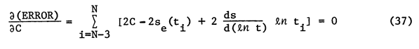
and
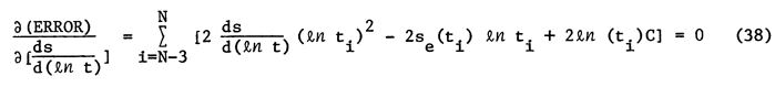
Solving these two equations simultaneously gives
The results expressed by equations (39) and (40) can now be used in equations (30) and (35) to calculate an initial guess for T and S when needed. This procedure works well if the restrictions on r and t are observed.
Appendix I contains a listing of program THEIS, a time-sharing FORTRAN program for evaluation of equation (1). In addition to drawdown (s), the program will print out the quantity u = r2S/4Tt, the well function W(u), and the sensitivity coefficients given by equations (13) and (14). The gal-day-foot system or any consistent set of units may be used.
Figure 1 is a printout of a typical run. The user's response is underlined. The program initiates a series of questions after the RUN command is typed and a carriage return is given. A carriage return is required after each response. The first question asks if the user wants u, W, and the sensitivity coefficients printed. Any response other than YES with no leading or imbedded blanks is interpreted as NO. All other questions requiring a YES or NO answer are similar. In Figure 1, the extra printout was requested. The second question defines the system of units. The user can use the gal-day-foot system or any consistent set of units. A YES response, as in Figure 1, means the gal-day-foot system is being used.
Figure 1--Typical run of program THEIS.
DO YOU WANT U, W, AND SENSITIVITY VALUES PRINTED ?
=YES
DO YOU WANT TO USE THE GAL, DAY, FT SYSTEM ?
=YES
STORAGE COEFFICIENT (UNITLESS)
=.001
TRANSMISSIVITY (GAL/DAY/FT) OR (L**2/T)
=24000
CONSTANT PUMPAGE (GAL/DAY) OR (L**3/T)
=240000
CONSTANT OBSERVATION POINT?
=YES
CONSTANT OBSERVATION TIME?
=NO
OBSERVATION POINT (FT) OR (L)
=100
OBSERVATION TIME (DAYS) OR (T)
=.001
THE DRAWDOWN IS           0.25669954
U = 0.77916666E 00
W = 0.32257789E 00
SENSITIVITY WITH RESPECT TO TRANSMISSIVITY =           0.45163666E-05
SENSITIVITY WITH RESPECT TO STORAGE =           -0.3650q233E 03
OBSERVATION TIME (DAYS) OR (T)
=.01
THE DRAWDOWN IS           1.63239339
U = 0.77916667E-01
W = 0.20513243E 01
SENSITIVITY WITH RESPECT TO TRANSMISSIVITY =           -0.37344505E-04
SENSITIVITY WITH RESPECT TO STORAGE =           -0.73612525E 03
OBSERVATION TIME (DAYS) OR (T)
=.1
THE DRAWDOWN IS           3.41010541
U = 0.77916667E-02
W = 0.42852612E 01
SENSITIVITY WITH RESPECT TO TRANSMISSIVITY =           -0.10918776E-03
SENSITIVITY WITH RESPECT TO STORAGE =           -0.78959904E 03
The program states the acceptable units for each parameter as the user is asked to type in the value. L is any arbitrary length unit and T is any arbitrary time unit. A unitless storage coefficient of .001 has been used in Figure 1. Transmissivity in units of gal/day/ft or L2/T must be specified. A value of 24,000 gal/day/ft has been used in the example. A constant pumpage of 240,000 gal/day has been used in Figure 1. In consistent units, pumpage must be specified in units of L3/T.
At this point two more yes-no questions are asked. The first asks if the user wants a constant observation point, making r in equation (1) constant for this run. This is the normal situation when one observation well is used to measure water levels as a function of time. The next question concerns time. Is t in equation (1) to be held constant for this run? This would be the situation if one measured the drawdown at the same time in a number of observation wells. If the answer to both questions is YES, the program accepts only one value of r and t, calculates the desired quantities, and then terminates. If only one of the questions is answered YES, the program continues to ask for updated values of the parameter that is not constant. In Figure 1, time is not constant so the program continually asks for new times. To terminate the program, the user simply hits the BREAK button. If both questions are not YES, then the program asks for updated values of both r and t until the BREAK button is pushed. In Figure 1, a constant r of 100 feet has been specified while several times have been given ranging from .001 days to .1 days.
Appendix II contains a listing of subroutine THEIS. It is a FORTRAN IV subroutine for the evaluation of equations (1), (13), and (14) that can be incorporated into any user deck and called by the mainline program. To employ subroutine THEIS, the user simply includes the following call statement at the appropriate place in the mainline program:
CALL THEIS(SC, KB, Q, R, T, S, DSDT, DSDSC, UNIT).
The parameters SC, KB, Q, R, T, and UNIT must be assigned a value or character designation prior to calling THEIS. SC is the unitless storage coefficient. UNIT must be declared a character type of variable in the mainline program. If the user wishes to use the gal-day-ft system, UNIT must be set to 3HYES in the mainline. Any other character string is interpreted as NO and the subroutine assumes a consistent set of units. KB is the transmissivity (gal/day/ft or L2/T), Q is the constant pumpage (gal/day or L3/T), R is the distance of the observation well from the pumped well (feet or L), and T is the elapsed time since pumping started (day or T). The transmissivity KB should be declared REAL in the mainline since it would be implicitly typed INTEGER.
Upon returning to the mainline, parameters S, DSDT, and DSDSC have been assigned values by subroutine THEIS. These values represent the evaluation of equations (1), (13), and (14) respectively. S is the drawdown in units of feet or L. DSDT is the sensitivity coefficient with respect to transmissivity in units of ft2day/gal or T/L. DSDSC is the sensitivity coefficient with respect to storage in units of feet or L. Upon returning to the mainline, these three parameters are available to the user for printout or further computation. This subroutine is used in the next program to be discussed; the reader is referred there for an example of the usage of subroutine THEIS.
This program fits the Theis equation to experimental pumptest data to obtain the "best" values for the storage coefficient and the transmissivity by using a least squares procedure discussed earlier. The program exists in two forms: a time-sharing FORTRAN version and a FORTRAN IV batch version. The time-sharing version is listed in Appendix III and the batch version in Appendix IV. The two programs are basically identical except for data input.
Figure 2 is the printout of a typical time-sharing run. The user's response is underlined. As with program THEIS, this program initiates a series of questions after the RUN command is given with a carriage return. The first question defines the system of units. YES allows use of the gal-day-foot system; any other response is interpreted as NO. Because NO was the response in Figure 2, a consistent set of units is assumed. The second question asks if the user wishes to make an initial guess for the storage and transmissivity. In Figure 2, NO was given, so no input for these quantities was required. If the response had been YES, the program would have requested the user to type in the guesses for storage and transmissivity in the two following questions. In Figure 2, the pumpage rate is given as 66.07 ft 3 /min. The observation well was located 545 feet from the pumped well. The next question asks how many drawdown-time pairs are to be read into the program. In this case it is 18. At this point the program echo prints all data typed in thus far. This allows error checking. Since guesses for storage and transmissivity were not given, they are printed as zero. SC stands for storage coefficient and KB for transmissivity.
Figure 2--Typical run of program THEISFIT (time sharing version).
DO YOU WANT TO USE GAL, DAY, FT SYSTEM ?
=NO
GUESS FOR STORAGE AND TRANSMISSIVITY ?
=NO
CONSTANT PUMPAGE RATE ? GAL/DAY OR L**3/T
=66.07
OBSERVATION DISTANCE FROM PUMPING WELL ? FT OR L
=545
NUMBER OF DFAWDOWN-TIME PAIRS TO BE READ ?
=18
ECHO THE INITIAL DATA
SC = 0.             KB = 0.
Q = 0.66070000E 02 R = 0.54500000E 03 N = 18
TYPE IN DRAWDOWN-TIME PAIRS IN ORDER OF INCREASING TIME.
=.02,50
=.05,60
=.08,70
=.13,80
=.18,90
=.22,100
=.33,120
=.43,140
=.54,160
=.64,180
=.74,200
=.94,240
=1.12,280
=1.30,320
=1.47,360
=1.66,400
=1.92,460
=2.17,535

THE PUMP TEST DATA IN DRAWDOWN-TIME PAIRS
     0.200000OOE-01      0.50000000E 02
     0.500000OOE-01      0.60000000E 02
     0.800000OOE-01      0.70000000E 02
     0.13000000E 00      0.80000000E 02
     0.18000000E 00      0.90000000E 02
     0.22000000E 00      0.10000000E 03
     0.33000000E 00      0.12000000E 03
     0.43000000E 00      0.14000000E 03
     0.54000000E 00      0.16000000E 03
     0.64000000E 00      0.18000000E 03
     0.74000000E 00      0.20000000E 03
     0.94000000E 00      0.24000000E 03
     0.11200000E 01      0.28000000E 03
     0.13000000E 01      0.32000000E 03
     0.14700000E 01      0.36000000E 03
     0.16600000E 01      0.40000000E 03
     0.19200000E 01      0.46000000E 03
     0.21700000E 01      0.53500000E 03
THE CALCULATED GUESS FOR KB AND SC IS    0.29628059E 01   0.35149625E-02
BEST FIT KB AND SC THIS ITERATION ARE    0.25232340E 01   0.46495635E-02
BEST FIT KB AND SC THIS ITERATION ARE    0.22588631E 01   0.47946684E-02
BEST FIT KB AND SC THIS ITERATION ARE    0.22523235E 01   0.47765156E-02
BEST FIT KB AND SC THIS ITERATION ARE    0.22523887E 01   0.47765839E-02
THE BEST FIT DRAWDOWN-TIME PAIRS
     0.25206927E-01      0.50000000E 02
     0.49396171E-01      0.60000000E 02
     0.81189803E-01      0.70000000E 02
     0.11926181E 00      0.80000000E 02
     0.16227960E 00      0.90000000E 02
     0.20906690E 00      0.10000000E 03
     0.31022453E 00      0.12000000E 03
     0.41701533E 00      0.14000000E 03
     0.52587939E 00      0.16000000E 03
     0.63457878E 00      0.18000000E 03
     0.74181844E 00      0.20000000E 03
     0.94917238E 00      0.24000000E 03
     0.11451357E 01      0.28000000E 03
     0.13292893E 01      0.32000000E 03
     0.15021422E 01      0.36000000E 03
     0.16645316E 01      0.40000000E 03
     0.18904877E 01      0.46000000E 03
     0.21471107E 01      0.53500000E 03
THE RMS ERROR FOR DRAWDOWN IS   0.17307440E-01
The program is now ready to accept drawdown-time pairs. They should be read in order of increasing time since the last four are used to calculate an initial guess for storage and transmissivity. The guess-calculating routine assumes these four are at large values of time. If the user supplies an initial estimate for storage and transmissivity, the drawdown-time pairs may be read in any order. Notice that the drawdown must be typed first and the time second with a separating comma. The values may be typed with or without a decimal point and may be in scientific notation (for example, 1.3 x 10⁵ would be typed 1.3E5). After the 18 pairs have been typed, the program echo prints them for error checking.
From this point on, the user may not interact with the program. One of two things should now happen: the program will converge to the "best" solution or the program will not converge. If it does not converge after 20 iterations, the program terminates. However, if the initial guess for storage and transmissivity was bad or if the data are rather poor, unphysical values for storage and transmissivity or error messages may be generated in the iteration process. If this occurs, the program may be terminated by hitting the BREAK key. In general, the storage and transmissivity guesses may be overestimated or underestimated by two or three orders of magnitude and still achieve convergence.
In the example shown in Figure 2, the calculated guess is printed first, followed by a series of iterations. The current "best" fit is printed for each iteration. Convergence is achieved in four iterations in this example. The convergence criteria requires the change in storage and transmissivity since the last iteration to be less than or equal to .1%. The program proceeds to print the "best" fit drawdown-time pairs and calculates the rms error in the drawdown. The rms error is a measure of the absolute error at an "average" data point. In this example, one would expect the "average" difference between measured and calculated drawdown to be about .017 feet.
The data set for a typical run of the batch version of THEISFIT is shown in Figure 3. The first card must contain values for the two character variables GUESS and UNIT. YES or NO are the appropriate responses. The first variable is GUESS. Its value must start in column one. YES means that the user is going to supply the first guess for storage and transmissivity. The second variable, UNIT, must start in column seven. YES means the user wants to use the gal-day-foot system. Any other response indicates a consistent set of units is being used. In this particular example, an initial guess for SC and KB is given and the gal-day-foot system is used.
Figure 3--Typical data set for batch version of THEISFIT.
YES   YES
    .00001      2000    316800       824        22
        .3   .002083        .7   .003472       1.3   .005556       2.1   .008333
       3.2   .013889       3.6   .016667       4.1   .020833       4.7   .026389
       5.1   .032639       5.3   .034722       5.7   .041667       6.1   .048611
       6.3   .055556       6.7   .062500       7.0   .069444       7.5   .090278
       8.3   .111111       8.5   .138889       9.2   .180556       9.7   .222222
      10.2   .263889      10.9   .347222
The next card contains five variables: storage (SC), transmissivity (KB), pumpage (Q), observation distance (R), and the number of drawdown-time pairs to be read (N). These variables are read under a (4F10.0, I10) format. Each variable field is ten columns wide. The first four variables may be punched with or without a decimal point; however, if no decimal is punched it will be assumed to be at the extreme right of the field. If no decimal is punched, the value should be right justified. The last variable, N, must be right justified (ending in column 50) and punched without a decimal point. If GUESS is given as NO, the program ignores any values given for SC and KB on the second card. In this example SC is .00001, KB is 2,000 gal/day/ft, Q is 316,800 gal/day, R is 824 feet, and N is 22 pairs.
The drawdown-time pairs are punched on the third and following cards at a maximum of four pairs per card. The pairs are read under an (8F10.0) format. Each data field is ten columns wide. Decimal consideration is the same as for SC, KB, Q, and R. They should be punched in order of increasing time if a guess for SC and KB is to be calculated by the program. In this example, drawdowns are given in feet and time in days.
The output for the data set of Figure 3 is shown in Figure 4. The input data are printed out for error checking. Since GUESS was given as YES, no guess was calculated for SC and KB. The program converged in six iterations. The convergence criteria are the same as for the time-sharing version. Comments on the convergence properties of the time-sharing version also apply to the batch version. The best fit drawdown-time pairs are printed if convergence is obtained. The rms error for the drawdown is .091 feet for this example. Therefore, the "average" error in drawdown is .091 feet.
Figure 4--Output for a typical run of the batch version of THEISFIT.
ECHO THE INITIAL DATA
SC = 0.100000OOE-04 KB = 0.20000000E 04
Q = 0.31680000E 06 R = 0.82400000E 03 N =   22
THE PUMP TEST DATA IN DRAWDOWN-TIME PAIRS
     0.30000000E 00         0.208300OOE-02
     0.70000000E 00         0.347200OOE-02
     0.13000000E 01         0.555600OOE-02
     0.21000000E 01         0.833300OOE-02
     0.32000000E 01         0.138890OOE-01
     0.36000000E 01         0.166670OOE-01
     0.41000000E 01         0.208330OOE-01
     0.47000000E 01         0.263890OOE-01
     0.51000000E 01         0.326390OOE-01
     0.53000000E 01         0.347220OOE-01
     0.57000000E 01         0.416670OOE-01
     0.61000000E 01         0.486110OOE-01
     0.63000000E 01         0.555560OOE-01
     0.67000000E 01         0.625000OOE-01
     0.70000000E 01         0.694440OOE-01
     0.75000000E 01         0.902780OOE-01
     0.83000000E 01         0.11111100E 00
     0.85000000E 01         0.13888900E 00
     0.92000000E 01         0.18055600E 00
     0.97000000E 01         0.22222200E 00
     0.10200000E 02         0.26388900E 00
     0.10900000E 02         0.34722200E 00
BEST FIT KB AND SC THIS ITERATION ARE      0.36231568E 04  0.15993002E-04
BEST FIT KB AND SC THIS ITERATION ARE      0.59841841E 04  0.21295657E-04
BEST FIT KB AND SC THIS ITERATION ARE      0.84381630E 04  0.22418721E-04
BEST FIT KB AND SC THIS ITERATION ARE      0.97266890E 04  0.21174726E-04
BEST FIT KB AND SC THIS ITERATION ARE      0.99078571E 04  0.20944681E-04
BEST FIT KB AND SC THIS ITERATION ARE      0.99086274E 04  0.20949939E-04
THE BEST FIT DRAWDOWN-TIME PAIRS
     0.35065781E 00      0.208300OOE-02
     0.82974025E 00      0.347200OOE-02
     0.14774877E 01      0.555600OOE-02
     0.21714489E 01      0.833300OOE-02
     0.31821451E 01      0.138890OOE-01
     0.35709338E 01      0.166670OOE-01
     0.40622920E 01      0.208330OOE-01
     0.45985823E 01      0.263890OOE-01
     0.50920417E 01      0.326390OOE-01
     0.52373781E 01      0.347220OOE-01
     0.56696365E 01      0.416670OOE-01
     0.60390812E 01      0.486110OOE-01
     0.63617290E 01      0.555560OOE-01
     0.66480276E 01      0.625000OOE-01
     0.69053687E 01      0.694440OOE-01
     0.75506012E 01      0.902780OOE-01
     0.80648859E 01      0.11111100E 00
     0.86204649E 01      0.13888900E 00
     0.92767410E 01      0.18055600E 00
     0.97979766E 01      0.22222200E 00
     0.10230386E 02      0.26388900E 00
     0.10922440E 02      0.34722200E 00
THE RMS ERROR FOR DRAWDOWN IS       0.91011392E-01
The automated fit for pumptest data developed in this work should be a useful tool for the groundwater hydrologist. We have used it on many more pumptests than the two examples included here. It is simple to use, quick, and inexpensive. The automated fit has the advantage that it is always objective. As a measure of the error in fitting, the rms error in drawdown is calculated for the "best" transmissivity and storage. For the cases we have run, the rms error in drawdown is no more than a few tenths of a foot. If it is much larger than this, one has either poor data or a hydrologic situation that cannot be represented by the Theis equation.
The algorithm for fitting has good convergence properties. Convergence is generally achieved even if the initial guess is too large or too small by two or three orders of magnitude. The procedure has been tested over a wide range of transmissivity and storage.
This work deals only with the Theis equation. However, sensitivity analysis and least squares fitting could be applied to more hydrologically complicated situations. Automated fitting routines could be developed for such common situations as anisotropic flow, partial penetration, leaky aquifers, delayed yield, and hydrologic boundaries.
Abramowitz,, M., and Stegun, I.A., 1968, Handbook of mathematical functions: New York, Dover Publications, p. 231.
Carnahan, B., Luther, H.A., and Wilkes, J.O., 1969, Applied numerical methods: New York, John Wiley, p. 571-573.
Hildebrand, F.B., 1962, Advanced calculus for applications: Englewood Cliffs, Prentice-Hall, p. 360.
Jacob, C.E., 1940, The flow of water in an elastic artesian aquifer: Transactions of the American Geophysical Union, v. 21, p. 574-586.
Jacob, C.E., 1950, Flow of groundwater; in, Rouse, H., ed., Engineering hydraulics: New York, John Wiley, p. 343.
McCuen, R.H., 1973, Component sensitivity: a tool for the analysis of complex water resources systems: Water Resources Research, v. 9. no. 1. p. 243-246.
McElwee, C.D., and Yukler, M.A., 1978, Sensitivity of groundwater models with respect to variations in transmissivity and storage: Water Resources Research, v. 14, no. 3, p. 451.
Theis, C.V., 1935, The relation between the lowering of the piezometric surface and the rate and duration of discharge of a well using groundwater storage: Transactions of the American Geophysical Union, v. 16, p. 519-524.
Tomovic, R., 1962, Sensitivity analysis of dynamic systems: New York, McGraw-Hill, 141 p.
Vemuri, V., Dracup, J.A., Erdmann, R.C., and Vemuri,, N., 1969, Sensitivity analysis method of system identification and its potential in hydrologic research: Water Resources Research, v. 5. no. 2, p. 341-349.
Yukler, M.A., 1976, Analysis of error in groundwater modelling: Ph.D. dissertation, The University of Kansas, 182 p.
Next Page--Appendices with Source Code
Kansas Geological Survey, The Theis Equation
Placed on web June 18, 2012; originally published in 1980.
Comments to webadmin@kgs.ku.edu
The URL for this page is http://www.kgs.ku.edu/Publications/Bulletins/GW3/index.html