Kansas Geological Survey, Bulletin 233, p. 335-344
by
Maurizio Ripepe1 and Alfred G. Fischer2
1University of Florence
2University of Southern California
Previous work on a pelagic stratigraphic sequence in the Middle Cretaceous (Albian) of Italy, about 100 Ma, defined a hierarchy of oscillations. These were identified as variations in carbonate productivity and bottom fauna linked to seafloor aeration. The sequence geometry suggests response to orbitally driven climatic variations, reflecting Berger's precession index, which depicts the precession cycle as a carrier wave modulated by orbital eccentricity. Here we use Berger's astronomic precession index curve for the past 1,500 k.y. in combination with the stratigraphic data to construct a forward model of sedimentation and stratigraphy. The precession index curve serves as a point of departure, and modeling proceeds in three steps: (1) conversion of the precession index into a curve of sedimentation rates through time, using the flux rates calculated from the stratigraphy and applied in a nonlinear way; (2) conversion of that curve into an ideal stratigraphy in which the time dimension is changed into the spatial dimension of stratigraphy; and (3) modification of this stratigraphy by bioturbation as a nonlinear function of seafloor aeration. This computer simulation produces a reasonably good match to the observed stratigraphy. Perhaps more important is the insight gained into changes in the distribution of spectral power; whereas the power of the precession index lies wholly in the precessional terms, that of the stratigraphic sequence lies largely in the eccentricity frequencies. Our model shows how power is transferred from one to the other in each of the three steps. The spectrum of the ultimate stratigraphy synthesized is essentially identical with that of the natural sequence.
An Acrobat PDF file containing the complete paper is available (724 kB).
Concern with stratigraphic cyclicity goes back a century (Gilbert, 1895). In the beginning this interest was largely centered on repetitions of strata observed in the field. Recent studies have introduced instrumental scans of cores and boreholes or chemical profiles based on closely spaced analyses (Fischer et al., 1990). Such studies permit calculation of flux rates and lend themselves to modeling.
The Aptian-Albian Scisti a Fucoidi (Arthur and Premoli Silva, 1982; Tomaghi et al., 1989) is a cyclically stratified sequence of pelagic marls in the Umbrian facies of central Italy. DeBoer and Wonders (1984) interpreted these cycles as expressions of climatic oscillations linked to orbital forcing (precession and eccentricity), as worked out for glacial cycles of the Pleistocene (Berger, 1977a,b; Berger et al., 1988; Imbrie, 1982; Imbrie et al., 1984). A core cut through the entire formation at Piobbico, by Premoli Silva, Napoleone, and Fischer (Herbert and Fischer, 1986; Tomaghi et al., 1989), allows instrumental analyses and scans of the entire sequence in a fresh state. Studies of that core are still in progress. Herbert and Fischer (1986) and Herbert et al. (1986) analyzed a 1,600-k.y. segment of the core from the Ticinella praeticinensis zone by means of physical and chemical profiles. They confirmed the earlier interpretations of orbital control. The cyclicity resulted from a double oscillation: one in seafloor aeration and the other in pelagic carbonate production. The orbital timing permitted calculation of mean flux rates.
In this study we assume that the interpretations of deboer and Wonders and of Herbert and Fischer are correct: Seafloor aeration and pelagic carbonate production were related to the orbital variations. We invert this deduction in a forward model, attempting to derive a stratigraphy from the astronomical precession index curve by assuming that the observed geologic oscillations are simple functions of that curve.
It should be clear from the outset that we do not imply a direct response of sedimentation to the orbitally driven variations in insolation patterns. Such responses must have occurred by roundabout pathways involving atmospheric climate and the oceans. Each response is likely to be nonlinear and accompanied by feedback (Imbrie and Imbrie, 1980; Imbrie, 1982). But, because we are unable to model atmospheric and oceanic responses and at the risk of being naive, we have leaped over these obstacles in a pragmatic attempt to model the sedimentation and stratigraphy of a 1,600-k.y. sequence, almost 100 Ma, from the astronomical insolation curves (precession index) of our time. In developing this model, we had only two variables to work with, both involving nonlinearity in response to orbital forcing; the nonlinearity in the response of carbonate production and the nonlinearity in the response of bioturbation. A simple formula sufficed to provide a synthetic stratigraphy quite similar to that observed.
Our model demonstrates the potential of bioturbation to overprint original depositional cyclicities. It also illuminates the long-standing problem of why geologic phenomena such as ice volume and bedding rhythms have such a prominent 100-k.y. eccentricity signal by showing how each nonlinear step transfers power from the precession (carrier wave) to the eccentricity (modulator waves).
The Scisti a Fucoidi (Fucoid Marls) in the central Apennines of Italy represents pelagic carbonate-clay oozes deposited slowly on the slope leading from the carbonate platforms of the Apulian promontory (presumably linked to Africa) to the Ligurian trough (Arthur and Premoli Silva, 1982). The biota consists largely of coccoliths and planktonic foraminifers and yields the full complement of Aptian-Albian zones (Tomaghi et al., 1989). Absence of shells or molds of aragonitic fossils implies deposition below the aragonite compensation depth and suggests water depths of 1-2 km (3,000-6,000 ft). Absence of graded bedding and sole marks and the consistency of stratification patterns suggest continuous sedimentation patterns that were only locally disturbed by stumps.
The strata show striking patterns of cyclicity. Low-carbonate-high-carbonate bedding couplets, averaging 10 cm (4 in.) thick, are obvious in the outcrop. The couplet members are distinguished by their weathering profiles (with the limestones forming more prominent and more massive ledges) and their color (with lightness being proportional to carbonate content). Such couplets are arranged into bundles of four to six, in which the central couplets are more calcareous and therefore lighter and thicker than the marginal ones, which commonly contain one or two thin black shales.
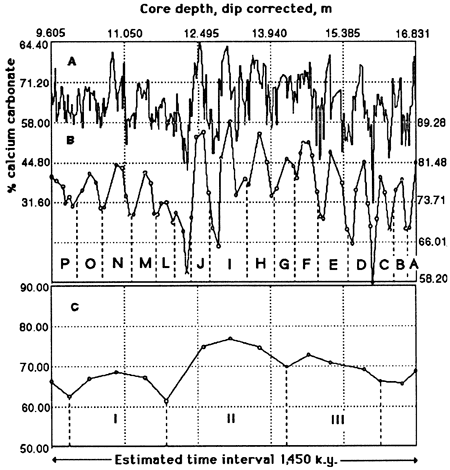
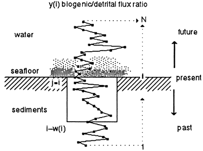
A core drilled through the Scisti a Fucoidi at Le Brecce near Piobbico (Tomaghi et al., 1989) is still under study. A segment of this core from the T. praeticinensis subzone has been studied in detail (Herbert and Fischer, 1986; Herbert et al., 1986). The distribution of calcium carbonate in 7.22 m (23.7 ft) of strata is shown in fig. 1A. There are 74 high-frequency digitations, but elimination of those peaks based on only one data point reduces the number to 68. These are the bedding couplets, which in this core average 10.6 cm (4.2 in.) thick.
Reducing these data to couplet means (fig. 1B) demonstrates the grouping of couplets, in sets of 4 or 5, into bundles, of which there are 15, averaging 48.2 cm (19.0 in.) thick.
Further reducing these numbers to bundle means (fig. 1C) demonstrates a grouping of these bundles into 4 superbundles, averaging 93 cm (37 in.) thick.
Figure 1--Calcium carbonate percentages of Piobbico core segment. (A) Raw carbonate percentages [after Herbert and Fischer (1986)]. The high-frequency oscillations correspond to the bedding couplet inferred to represent the 20-k.y. precessional signal. (B) Mean carbonate percentages calculated for couplets. The curve has not been smoothed and defines 15 cycles corresponding to the bundles observed in the field and attributed to the 100-k.y. eccentricity cycle. (C) Mean carbonate percentages calculated for bundles as defined in part B. This unsmoothed curve defines 3.5 cycles (superbundles) attributed to the 400-k.y. eccentricity cycle.
It is tempting to consider these regular hierarchical oscillations as responses to a hierarchy of rhythmic forcing functions that operate through climate and oceanic behavior. What were their periods? Like the durations of most Mesozoic stages, the duration of the Albian is only loosely constrained by radiometric dates (Harland et al., 1982). Recent estimates (Cowie and Bassett, 1989) range from 12 m.y. to 17 m.y. Because the top of the Albian lies several meters above the base of the succeeding Scaglia Bianca Limestone, the 43 m (140 ft) of Albian deposits in the Piobbico core (Tomaghi et al., 1989) represents slightly less than the full span, say, 10-14 m.y. That implies a mean rock accumulation rate of 3.1-4.3 Bubnoff units (m/m.y. or mm/k.y.).
But was the core segment deposited at the mean rate? It is notably more calcareous than the middle part of the Scisti a Fucoidi (Tomaghi et al., 1989), where dissolution features suggest greater loss of carbonate by seafloor dissolution. Also, the upper part of the formation is transitional to the Scaglia Bianca Limestone. Assuming a duration of 4-6 m.y. for the Cenomanian, the rock accumulation rate for the Scaglia Bianca is 9-14 Bubnoff units. We thus conclude that the T. praeticinensis subzone was deposited at a rate somewhat higher than the average for the Scisti a Fucoidi and that the 5-Bubnoff rate assumed by Herbert and Fischer (1986) is a reasonable compromise.
According to that rate, the couplets have a mean period of 21 k.y., the bundles a mean period of 98 k.y., and the superbundles a mean period of 400 k.y. These frequencies match those of the precession and the shorter and longer eccentricity cycles (Berger, 1978).
These frequencies find support in spectral analysis. Although the carbonate curve shows no power (see fig. 5E) above noise level for the precession and obliquity periods, it shows major peaks at 92.5 k.y. and 115.7 k.y., corresponding to the astronomical eccentricity modes at 94 k.y. and 123 k.y. This is confirmed by the more sophisticated analysis of Park and Herbert (1987), which also brings out a periodicity at 39 k.y. and is a likely candidate for the obliquity cycle. The 400-k.y. eccentricity cycle is not apparent in the spectrum, but a peak at a nominal 694 k.y. (poorly constrained because of the logarithmic scale) may be the 800-k.y. double of this cycle.
Subsequent analyses of a somewhat longer [10-20 m (3060 ft)] interval by Premoli Silva, Ripepe, and Tomaghi (1989) have also demonstrated the orbital frequencies: A spectrum for foraminiferal abundance shows a 44-k.y. peak that may represent the obliquity and a prominent 111-k.y. peak for the eccentricity as well as the 800-k.y. peak.
Orbital frequencies are also apparent in detailed magnetic data (intensity, inclination, and declination) obtained for a 2-m (7-ft) segment of core from the same zone (Napoleone and Ripepe, 1989). Presumed precessional peaks lie at 17 k.y. and 19 k.y. in the spectrum for magnetic intensity and at 17 k.y. in the inclination spectrum. A 26-k.y. peak on the inclination spectrum remains unassigned. Peaks attributed to obliquity appear in the range 38-42 k.y. in all 3 spectra, and all spectra show a dominant eccentricity peak at 105 k.y. Further magnetic work is in progress.
The chronology thus obtained made it possible for Herbert and Fischer (1986) and Herbert et al. (1986) to convert percentages of carbonate and silicate couplet means into flux rates of biogenic and detrital matter (figs. 2 and 3). Assuming that carbonate cement is derived from biogenic carbonate, all carbonate is ascribed to pelagic biogenic origin. A siliceous biogenic fraction, calculated theoretically from the silica excess in relation to aluminum, amounts to 8% of carbonate. As shown in fig. 3, the detrital flux varied between 0.1 g/cm2/k.y. and 0.6 g/cm2/ k.y., whereas the biogenic flux varied between 0.1 g/cm2/k.y. and 2.5 g/cm2/k.y. These fluxes are positively correlated, but the variation in detrital flux is small. As already shown by deboer and Wonders (1984) from the correspondence of couplet thickness to carbonate content, the cycle is primarily a carbonate productivity cycle.
Figure 2--Mean flux rates of (A) detritus and (B) biogenic matter for the couplets plotted against thickness. Detrital and biogenic flux rates varied in parallel, but the detrital variation is small compared to that of the biogenic fraction; the cycles are productivity cycles.
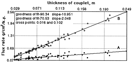
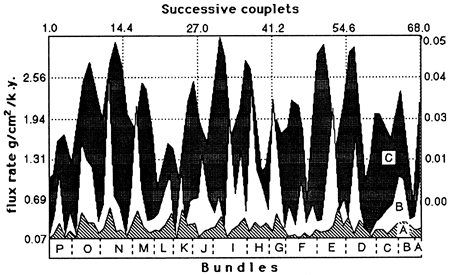
Figure 3--Flux rates (couplet means) of (A) detritus and (B) biogenic matter compared to (C) the eccentricity cycles astronomically calculated for the interval 1,450 k.y. B.P. to 150 k.y. A.P.
Carbon isotope ratios are consistently displaced to the positive side from adjacent shales (deboer and Wonders, 1984), contrary to what would be expected from diagenetic (cementation) overprints. This offers further evidence that limestones mark the times of higher productivity and shales the times of lower productivity. This is particularly true for the lean (hydrogen-deficient) black shales of this core segment. It is not true for the hydrogen-rich black shales that occur lower in the sequence; these shales record productivity peaks (Premoli Silva, Erba, and Tomaghi, 1989).
If Herbert and Fischer's (1986) carbonate curve reflects a cycle in carbonate productivity, then their curve of darkness, obtained by densitometry of diapositive photographs of the core, reflects another factor-bottom aeration. Black and somewhat laminated shales are devoid of trace fossils (except where penetrated by Chondrites from above) and mark times when the bottom was devoid of macroscavengers, presumably because of lack of oxygen. Succeeding drab marls are generally replete with the dysaerobic trace fossil Chondrites, the "fucoids" from which the formation derives its name. The succeeding whitish limestones are thoroughly bioturbated by Planolites and other coarse burrowers and were deposited on aerated bottoms. Individual burrows can reach a depth of 12 cm (4.7 in.) (compacted rock). This is a redox cycle much like the one described by Savrda and Bottjer (1989) from the Niobrara chalks and limestones of Colorado.
We can therefore infer not only a change in the number and type of burrowing animals but also a change in the manner, rate, and depth of burrow mixing. During times of anoxia, the bottoms were devoid of animals. Periods with a bit of free oxygen probably brought microscavengers that blurred the lamination without leaving visible burrows, the normal fabric of the black shales. Somewhat more oxygen brought sparse colonization by Chondrites. Although that enigmatic animal may have burrowed to some depth, it did so in soupy, now highly compacted sediment, and its shafts are now broadly splayed out on bedding planes. Further aeration brought a more diverse fauna of larger and more vigorous burrowers and less compactible carbonate ooze and resulted in more thorough bioturbation, with burrows extending up to 12 cm (5 in.) into compacted limestone.
The sedimentary system was thus governed by the interaction of oscillations in productivity and in seafloor aeration (redox), and these cycles were generally linked, with aeration corresponding to increased productivity. We note in passing that this linkage is not obligatory; carbonate content oscillates rhythmically in continuously red (i.e., oxidized) sediments in deeper parts of the sequence (Herbert, personal communication, 1989). The major control over these oscillations appears to have been exercised by the 20-k.y. precessional cycle and the 100-k.y. and 400-k.y. eccentricity cycles. These are the cycles to which we turn in modeling.
We aimed specifically at modeling the 7.22-m (23.7-ft) core segment for which Herbert and Fischer (1986) provided a calcium carbonate profile based on analyses with a mean spacing of 2 cm (0.8 in.) (4 k.y.). Because the main cycles expressed were those of the precession and the eccentricity, we ignored. the obliquity cycle and used Berger's climate precessional parameter (Berger, 1977a, 1978,1988) or precession index (Imbrie et al., 1984):
![]()
where e is the eccentricity and pi is the longitude of the perihelion as measured from the moving vernal equinox. This expresses nondimensionally the changes in insolation to be expected for a given latitude from the combination of precession (the carrier cycle) and the 100-k.y. and 400-k.y. cycles in orbital eccentricity (the modulators) (fig. 4A). The effect might be expected to be strongest in the middle latitudes. The horizontal midline corresponds to climates of average seasonality. Deviations from it imply, on the one side, deviations toward a greater seasonality (warmer summers and colder winters) and, on the other side, deviations toward reduced seasonality (cooler summers and warmer winters). These deviations are timed by the precession but vary in amplitude in proportion to orbital eccentricity.
Figure 4--The four steps in our computer simulation. (A) Precession index curve for the interval 1,450 k.y. B.P. to 150 k.y. A.P.; algorithm from Berger (1978). (B) Accumulation rate through time, obtained by varying biogenic flux rate as a logistic function of precession index. (C) Accumulation rate curve converted to a stratigraphy. Time axis of part B is converted to stratigraphic (space) dimension by adjustment to accumulation rate. Because accumulation rate is essentially governed by biogenic (skeletal) flux, the curve is a proxy for a primary stratigraphy in which the peaks are limestone and the troughs are shales. (D) Burrow mixing to depths varying from 0 to 12 cm (compacted rock) selectively converts many of the shales to marls.
We reiterate that the effects of such differences on atmospheric and oceanic circulation and of these on sedimentary settings must be complicated by nonlinear responses, lag times, feedback mechanisms, and interference between the hemispheres, which are out of phase with respect to the precession. We can predict neither direct nor indirect effects on marine productivity, oceanic structure, or turnover time. It seems, however, that changes in insolation patterns must have both direct and indirect effects on productivity. They are certain to change winds, especially the balance between zonal and monsoonal circulation, and thereby would drive changes in the patterns of upwelling and nutrient distribution. They might also affect the sites of oceanic bottom water formation and thereby the global oceanic circulation system, with widespread effects on oceanic stratification and turnover time. The close correspondence of late Pleistocene glacial history to the precession index also encouraged us in a direct modeling attempt.
Modeling had to begin with a specific segment of the precession index curve. Because our 7.22-m (23.7-ft) segment of stratigraphy was inferred to represent 1,450 k.y., we needed a segment of 1,600 k.y. of precession-eccentricity history that would be in phase with the geologic response. A time segment from 1,450 k.y. B.P. to 150 k.y. A.P. (Herbert and Fischer, 1986) provided an appropriate match between stratigraphic bundles and the astronomical eccentricity curve (fig. 3).
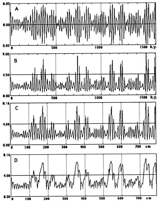
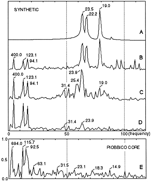
We begin with the precession index curve for 1,450 k.y. B.P. to 150 k.y. A.P. (Berger, 1977a), shown in fig. 4A. The power spectrum of this curve (fig. 5A) shows several precessional modes but no power in the eccentricity frequencies.
Figure 5--Amplitude spectra (fast Fourier transform) of (A) the precession index curve (see fig. 4A), (B) the accumulation rate curve (see fig. 4B), the primary stratigraphy (C) before bioturbation overprint (see fig. 4C) and (D) after bioturbation (see fig. 4D), and (E) the carbonate curve of the corresponding segment of Piobbico core (see fig. 1A).
Our working hypothesis was that the cyclicity observed in the rocks reflected (1) variations in carbonate productivity, yielding a complex curve of carbonate content, and (2) variations in bottom aeration, yielding variations in the depth of subsequent burrow mixing. Furthermore, we assumed both processes to be functions of orbital variations, as expressed in the selected segment of the precession index curve.
Accordingly, we modeled the process in two iterations, one designed to develop a primary stratigraphy and the other designed to produce the bioturbation overprint. Whether the flux rate of carbonate was a direct or inverse function of the precessional signal (i.e., whether maximal carbonate productivity occurred at maximal or minimal seasonality) was beyond our grasp and is immaterial to the model at its present stage.
The first modeling step involves the transformation of the precession index curve into a curve of detrital and biogenic sedimentary fluxes. The variation between these fluxes was expressed as a ratio of biogenic to detrital flux, which ranged from 0.72:1 to 9:1. Because detritus in the core showed only minor variations, it was modeled as a constant, supplied at a rate of 0.35 g/cm/k.y. or 1.27 mm/k.y. (compacted). This leaves the biogenic flux as the only variable.
The tentative premise that biogenic flux responds to orbital forcing as expressed in the precession index curve does not specify the function by which one is related to the other. Trial and error provided some guidelines. Assumption of a linear response produced far too much biogenic matter, yielding a stratigraphy far thicker than that observed. Would some simple nonlinear function provide the accumulations observed? A simple plot using the percentage of biogenic content, a highly nonlinear logistic function, provided an almost perfect match: a sedimentary sequence 7.94 m (26.0 ft) thick, only 0.8% short of the 8 m (26.2 ft) expected. Although there are presumably other nonlinear functions that would produce as good a match, we accept this function as pragmatically justified.
Because biogenic percentage values observed ranged from 42% to 90%, we identified the lowest precession index value with 42% and the highest with 90% and spaced the other percentage values arithmetically between these. Transforming these percentages into rock accumulation rates yields the curve of fig. 4B. This resembles the precession index curve (fig. 4A) but is asymmetric; nonlinear accumulation has shrunk the troughs and stretched the peaks. The Fourier spectrum of this curve is shown in fig. 5B.
In the second step we transformed the ordinate from the time base of the precession index into a stratigraphic base of meters of sediment by accumulating sediment according to
x(i) = (i - 1) + [y(I)dm + dm]dt, (2)
where x(i) is the stratigraphic (thickness) dimension, dm is the detrital accumulation constant (1.27 mm/k.y.), y(i) is the biogenic flux expressed as a factor of dm, and dt is the sampling rate of the precession index (2 k.y.).
The resulting ideal or primary stratigraphy (fig. 4C) has shale-limestone alternations for each precession but differs from that observed in nature by having many more black shales, with the most extreme ones occurring precisely where they are not observed-in alternation with the cleanest limestones. The corresponding amplitude spectrum is shown in fig. 5C.
In the third step we introduce bioturbation. As explained earlier, a complete redox cycle leads from no bioturbation in the black shale facies (less than 50% biogenic) through limited bioturbation in the Chondrites marls to thorough and deep burrow mixing in the Planolites facies of the limestones, to a maximum depth of 12 cm (4.7 in.) (compacted). For the sake of simplicity, we modeled bioturbation as a mixing process that occurs below the accreting surface of sedimentation to a depth that changes from 0 in the black shales (precession index troughs) to a maximum of 12 cm (4.7 in.) in the cleanest limestones (precession index peaks). Depth of bioturbation was modeled as the same logistic response assumed for the flux response of biogenic sedimentation. This was done by means of a traveling window within which sediments are homogenized (fig. 6). This window travels forward through time but looks backward, growing and shrinking between 0 and 12 cm (4.7 in.) in response to changing bottom aeration. The window is moved in 2-cm (0.8-in.) increments, and mixing is accomplished by averaging the sediment stepwise in two increments, expressed as
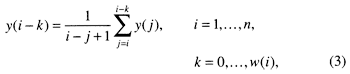
where y(i) is the sediment that is being bioturbated (fig. 4D) and w(i) is the window size.
Figure 6--Model of bioturbation. The seafloor moves upward through time by sediment accumulation. Burrow mixing below the seafloor is modeled by a window whose depth [w(i)] grows and shrinks with bottom aeration. Bottom aeration is reflected in the ratio of biogenic to detrital flux. In our model the window grows from 0 depth at a flux ratio of 1 to a maximal depth of 12 cm (compacted sediment) at a flux ratio of 9. Symbols defined in Eq. (3).
The backward-looking nature of this bioturbation process implies that the precessional signals will be best preserved when the precession index has low amplitude (low eccentricity), and burrow depth never grows large. As eccentricity and the amplitude of the precession index curve increase, bottoms become more anaerobic (less bioturbated) in one (10-k.y.) phase of the precessional cycle and more aerobic (more deeply bioturbated) in the other phase. At the low rates of sedimentation observed, the rapid increase in burrow-depth during increasing aeration destroys the preceding black shale, turning it into bioturbated marl. Thus the precessional signal becomes blurred at times of high eccentricity (figs. 4D and 5D).
This model was also tested by trial and error. A maximum burrow depth of 12 cm (4.7 in.) gave results most comparable to the natural sequence. A smaller window retained too many black shales; a larger one destroyed too much of the precessional (bedding couplet) record.
Figure 7 compares the natural carbonate curve of Herbert and Fischer (1986) with the synthetic one produced here. The gross characters, especially the occurrence of major limestones, are similar but displaced somewhat,just as the bundles in the core do not precisely match the eccentricity peaks of the precession index curve (fig. 3). This is not surprising inasmuch as the precession index curve never repeats itself precisely. The synthetic plot introduces too much carbonate into the shales, and shale distribution does not match in detail.
Figure 7--Calcium carbonate percentage curves. (A) Piobbico core segment. (B) Synthesized stratigraphy.
Spectral aspects Returning to the spectral domain (fig. 5), we recall first that the precession index has all its spectral power concentrated in the frequencies of the precession. This is due to the nature of spectra of modulated carrier waves, in which the symmetric nature of the modulating wave transfers its spectral power to the carrier. Imbrie and Imbrie (1980) showed for the Pleistocene how disturbances of such a record restore power to the modulator. The first step, conversion to a curve of accumulation rates in time (fig. 5B), yields small peaks for the 94-k.y. and 123-k.y. modes of the shorter eccentricity cycle and a peak for the 400-k.y. eccentricity cycle; precessional power is reduced accordingly. The second step, changing the time base to a stratigraphic base, further reduces and shifts the precessional peaks and increases the power of the eccentricity peak. The third step, bioturbation, brings further transfer of power from the precessional signals, which are now reduced to the level of noise, to the eccentricity frequencies. Indeed, the spectrum becomes virtually identical with that obtained from the carbonate profile of the natural sequence (fig. 5E).
We reiterate that our model, starting with relative changes in seasonal insolation patterns (precession index), does not follow the pathways through atmospheric and oceanic responses. It shortcuts these intermediate steps, currently beyond our grasp, to assume direct forcing of carbonate productivity (expressed in carbonate flux rates) and seafloor aeration (expressed in depth of bioturbation).
That is probably not realistic. There is every reason to expect that atmospheric response to orbital variations is nonlinear, as is oceanic response to insolation and atmospheric changes (Imbrie, 1982). The oceanic variations that drove both productivity and seafloor aeration probably had already acquired some power in the eccentricity frequencies. The percentage function we used may be more drastically nonlinear than what was actually exerted. But, even if our model is imperfect in placing the full burden of change on these last (geologic) steps, it has nevertheless served to identify the geologic processes that played a role and the general manner of their response.
Arthur, M. A., and Premoli Silva, I., 1982, Development of widespread organic carbon-rich strata in the Mediterranean Tethys; in, Nature and Origin of Cretaceous Carbon-Rich Facies, S. O. Schlanger and M. Cita,, eds.: Academic Press, New York, p. 8-54
Berger, A. L., 1977a, Long-term variation of the Earth's orbital elements: Celestial Mechanics, v. 15, p. 53-74
Berger, A. L., 1977b, Support for the astronomic theory of climatic change: Nature, v. 268, p. 44-45
Berger, A. L., 1978, A simple algorithm to compare long-term variations of daily or monthly insolation: Contribution 18, Institute d'Astronomie et de Geophysique G. Lemaitre, Universite Catholique de Louvain, Louvain-la-Neuve, Belgium
Berger, A. L., 1988, Milankovitch theory and climate: Reviews of Geophysics, v. 26, p. 624-657
Berger, A. L., Loutre, M. F., and Laskar, J., 1988, Insolation values for the climate of the last 10 Myr: Science Report 1988/13, Institute d'Astronomie et de Geophysique G. Lemaitre, Universite Catholique de Louvain, Louvain-la-Neuve, Belgium
Cowie, J. W., and Bassett, M. G., 1989, Global stratigraphic chart: Episodes, v. 12 (suppl.), 1 p.
deBoer, P., and Wonders, A. A. H., 1984, Astronomically induced rhythmic bedding in Cretaceous pelagic sediments near Moria (Italy); in, Milankovitch and Climate, A. L. Berger, J. Imbrie, J. Hays, G. Kukla, and B. Saltzman, eds.: Reidel, Dordrecht, p. 177-190
Fischer, A. G., deBoer, P., and Premoli Silva, I., 1990, Cyclostratigraphy; in, Cretaceous Resources, Events, and Rhythms, R. N. Ginsburg and B. Beaudoin, eds.: Kluwer Academic Publishers, Boston, Massachusetts, p. 134-172
Gilbert, G. K., 1895, Sedimentary measurement of geologic time: Journal of Geology, v. 3, p. 121-127
Harland, W. B., Cox, A. V., Llewellyn, P. G., Pickton, C. A. G., Smith, A. G., and Walters, R., 1982, A geologic time-scale: Cambridge University Press, Cambridge, 131 p.
Herbert, T. D., and Fischer, A. G., 1986, Milankovitch climatic origin of mid-Cretaceous black shale rhythms in central Italy: Nature, v. 329, p. 739-743
Herbert, T. D, Stallard, R. F., and Fischer, A. G., 1986, Anoxic events, productivity rhythms, and orbital signatures in a mid-Cretaceous deep-sea sequence from central Italy: Paleoceanography, v. 1, p. 495-506
Imbrie, J., 1982, Astronomic theory of the Pleistocene ice ages--a brief historical review: Icarus, v. 50, p. 408-422
Imbrie, J., and Imbrie, J. Z., 1980, Modeling the climatic response to orbital variations: Science, v. 207, p. 943-953
Imbrie, J., Hays, J., Martinson, D. G., MacIntyre, A., Mix, A. C., Morley, J. J., Pisias, N. G., Prell, W. L., and Shackleton, N. J., 1984, The orbital theory of Pleistocene climate-support from a revised chronology of the marine 180 record; in, Milankovitch and Climate, A. L. Berger, J. Imbrie, J. Hays, G. Kukla, and B. Saltzman, eds.: Reidel, Dordrecht, p. 269-305
Napoleone, G., and Ripepe, M., 1989, Cyclic geomagnetic changes in mid-Cretaceous rhythmites, Italy: Terra Nova, v. 1, p. 437-442
Park, J. J., and Herbert, T. D., 1987, Hunting for paleoclimatic periodicities in a geologic time-series with an uncertain time scale: Journal of Geophysical Research, v. 92, p. 14,027-14,040
Premoli Silva, I., Erba, E., and Tornaghi, M. E., 1989, Paleoenvironmental signals and changes in surface fertility recorded in mid-Cretaceous Corg-rich pelagic facies of the Fucoid Marls (central Italy): Geobios, Memoire Special, no. 2, p. 225-236
Premoli Silva, I., Ripepe, M., and Tomaghi, M. E., 1989, Planktonic foraminiferal distribution records productivity cycles--evidence from the Aptian-Albian of central Italy: Terra Nova, v. 1, p. 443- 448
Savrda, C. E., and Bottjer, D. J., 1989, Development of a trace-fossil model for reconstruction of paleo-bottom-water redox conditions--evaluation and application to Upper Cretaceous Niobrara Formation, Colorado: Paleogeography, Paleoecology, Paleoclimatology, v. 74, p. 49-74
Tornaghi, M. E., Premoli Silva, I., and Ripepe, M., 1989, Lithostratigraphy and planktonic foraminiferal biostratigraphy of the Aptian-Albian "Scisti a Fucoidi" in the Piobbico core, Marche, Italy--background for cyclostratigraphy: Rivista Italiana di Paleontologia e Stratigrafia, v. 95, p. 223-264
Kansas Geological Survey
Comments to webadmin@kgs.ku.edu
Web version April 21, 2010. Original publication date 1991.
URL=http://www.kgs.ku.edu/Publications/Bulletins/233/Ripepe/index.html