Kansas Geological Survey, Bulletin 233, p. 473-488
by
J. Fred Read1, David Osleger2, and Maya Elrick3
1 Virginia Polytechnic Institute and State University
2 University of Southern California
3 University of New Mexico
Two-dimensional stratigraphic models incorporating antecedent platform topography, rotational and regional driving subsidence, sediment and water loading using an elastic beam model, water-depth-dependent sedimentation rates and rock types, lag time of the flexural response, depositional lag time following initial platform flooding, and third- to fifth-order complex sea-level curves can be used to understand the development of cyclic carbonate platforms. Sea-level curves dominated by approximately 100-k.y. or 40-k.y. fluctuations developed a platform stratigraphy characterized by only a few cycles, whereas numerous cycles develop where the sea-level curve is dominated by 19-23 k.y. fluctuations. Low-amplitude sea-level curves in which the 100-k.y. fluctuation is greater than the 40-k.y. fluctuation, which in turn is greater than the 19-23-k.y. fluctuations, form a platform stratigraphy dominated by stacked cycles. Increased amplitude of the lower-frequency oscillations forms a shingled stacking pattern on the platform. Also, the increased amplitudes cause deposition of cycles with decreased thickness of tidal flat caps and longer duration of capping disconformities. Superimposing high-frequency sea-level fluctuations (20-100 k.y.) on longer-term 1-3-m.y. fluctuations generates synthetic platforms composed of stacked depositional sequences consisting of 1-10-m (3.3-33-ft) cycles. The model output illustrates how the systems tracts and their component cycles are related to the input sea-level curves. Erosion in the model decreases the thickness of tidal flat caps, increases the subtidal facies thicknesses of cycles because it increases accommodation, and bevels the highstand systems tract during long-term fall through erosion. The models show why picking boundaries between systems tracts is difficult when individual measured sections of cyclic platforms are used. Fischer plots were generated from the model output. The plots, when constructed for outer platform sections, are useful in estimating third-order sea-level fluctuations and in defining the positions of the systems tract boundaries.
An Acrobat PDF file containing the complete paper is available (1.4 MB).
Two-dimensional modeling is becoming widely used in simulations of carbonate platform stratigraphy. Some of these models simulate platforms at the seismic scale of complete basin fills, composed of numerous third-order sequences (Lerche et al., 1988; Aigner et al., 1988; Lawrence et al., 1990). These models tend to use subsidence and compaction algorithms involving tectonic subsidence and sediment and water loading, but sea-level curves dominated by third- and fourth-order sea-level fluctuations and long-term sedimentation rates that vary with position in the basin and that are of the same magnitude as long-term subsidence rates are also used. The models simulate stacked third-order depositional sequences and any internal fourth-order cyclicity but do not simulate the interrelated fourth- and fifth-order cyclic stratigraphy.
Other two-dimensional models concentrate on simulating fifth-order meter-scale cycle stratigraphy (Spencer and Demicco, 1989) or attempt to simulate platform geometries (Bice, 1988; Scaturo et al., 1989; Bosence and Waltham, 1990). These models tend to have sophisticated input sea-level curves and realistic carbonate sedimentation rates, but they ignore the important role of isostatic flexural response to loading. In this article we present a two-dimensional model that incorporates relatively complex sea-level curves, water and sediment loading using a flexural beam model, user-specified antecedent platform topography, short-term sedimentation rates (rather than long-term accumulation rates), lag times, and water-depth-dependent facies. The model generates stacked depositional sequences and their component fourth- and fifth-order cycles. The model does not provide a unique solution but can be used to evaluate the impact of individual input variables and can rapidly eliminate unreasonable combinations of variables. Except on rare carbonate platforms where the whole ramp to basin transition is completely exposed [e.g., Sarg (1988)], geologists cannot see in outcrop how groups of cycles relate to each other and to the systems tracts as a whole. Our model provides valuable clues related to the vertical and lateral relations of small-scale cycles bundled within systems tracts of carbonate ramps and the sequence- and cycle-bounding surfaces.
Total subsidence rates (long-term accumulation rates) are calculated from decompacted subsidence curves by dividing stratigraphic thickness (m) by duration (k.y.). Time is determined using the Decade of North American Geology (DNAG) time scale (Palmer, 1983). The endpoints of the interval of interest (e.g., Late Cambrian, Early Mississippian) are anchored so that all subsequent calculations remain consistent. Duration of a sequence is determined by
(s / S)T, (1)
where s is the thickness of the sequence, S is the thickness of the dated interval, and T is the total duration of the dated interval.
Minimum subsidence rates are calculated from the observed (nondecompacted) depth versus time curve. Tectonic subsidence rates for the outer edge of the platform are calculated from a best fit of the backstripped subsidence curve. Sections are backstripped using the procedure outlined by Watts and Ryan (1976) and Bond and Kominz (1984) and are based on
y = S* [(ρm - ρs) / (ρm - ρw)] + WD, (2)
where Y is the tectonic subsidence, S* is the delithified sediment thickness, ρm, ρs, and ρw are the densities of the mantle, sediment, and water, respectively, and WD is the estimated water depth of a lithofacies (generally ignored for shallow-water carbonates). As expected, tectonic subsidence rates are consistently calculated to be 30-40% of the total subsidence rate. Tectonic subsidence is considered to be linear over the short time intervals (1-3 m.y.) of the model runs.
Tectonic subsidence is divided into rotational and regional components for the modeling. Rotational subsidence is associated with rotation about a hinge line, as opposed to regional subsidence that is uniform across the platform. The partitioning of tectonic subsidence into two components is done by inspection of the gross cross-sectional geometry of the platform. The greater the wedge angle, the greater the amount of tectonic subsidence that is proportioned into the rotational component.
The subsidence resulting from local sediment and water loading is distributed across the platform according to the equations for loading of an elastic beam [modified from Jeffreys (1976)]:
ω = (σ / 2ρm)(eαx - cos αx) - (σ / 2ρm)[(eα(x-i) - cos α(x-1))] for -x, (3)
ω = (σ / 2ρm)(2-e-αx - cos αx) - (σ / 2ρm)[(2-e-α(x-i) - cos α(x-1))] for +x, (4)
where ω is total subsidence, x is the distance away from the edge of the load, i is the horizontal distance between localities, and α is a flexural parameter that is a function of beam rigidity:
![]()
where g is gravity and D is lithospheric rigidity. We let D equal 1032 dyne-cm, a value approximating a relatively mature passive margin. D is assumed to be constant over the relatively short 1-3 -m.y. durations of model runs. Because of edge effects, about 250 km (155 mi) on either side of the modeled platform are inaccurate and ignored in the interpretation of the model. (T is calculated by
(ρm)Δw + (ρs)Δs, (6)
where Δw is the change in the thickness of the water column and Δs is the change in the thickness of the sediment column [cf. Burton et al. (1987)].
Third-order (1-10 m.y.), fourth-order (100 k.y. to 1 m.y.), and fifth-order (<100 k.y.) sea-level curves used in the modeling can be input as symmetric or asymmetric sine waves or as a predetermined digitized curve. Magnitudes of third-order sea-level oscillations are estimated from Steckler and Watts (1978):
ΔSL = S* [(ρm - ρs) / ρm] - Y, (7)
where ΔSL is the change in sea level, S* is the delithified thickness of the sequence, ρm is the mean density of the mantle, ρs is the mean density of sediment, and Y is tectonic subsidence determined from backstripping (Moore et al., 1987; Bond et al., 1989). Magnitudes of sea-level changes estimated from inner platform sequence thicknesses will be underestimated because only part of the sea-level rise or fall is recorded. Estimates from deep ramp thicknesses must be corrected for the initial water depth in which the sediment was deposited (Steckler and Watts, 1978; Moore et al., 1987).
Third-order sea-level changes also can be roughly estimated from Fischer plots of peritidal capped cycles. Fischer plots graph cumulative cycle thickness (corrected for linear subsidence) against time of average cycle period (Fischer, 1964; Goldhammer et al., 1987; Read and Goldhammer, 1988). The plots define changes in accommodation space relative to the space created by linear subsidence. Changes in accommodation space may be due to short-term fluctuations in subsidence rate or eustatic sea-level fluctuations. Approximate magnitudes of sea-level fluctuations determined from isostatically corrected Fischer plots (Read and Goldhammer, 1988) can then be used in the modeling. The range of third-order rise and fall rates calculated by either method are similar to those calculated by Schlager (1981) and Haq et al. (1987) [<0.2 m/k.y. (<0.7 ft/k.y.)].
Short-term (<1 m.y.) sea-level fluctuations can be input as asymmetric or symmetric sine waves. For asymmetric sine waves, 15% of the period is taken in sea-level rise and 85% is taken in the fall, typical of glacio-eustatic sea-level signals (Hays et al., 1976). The periods of sea-level fluctuations can be determined from spectral analysis of subtidal cycles (de Boer, 1984; Arthur et al., 1984; Herbert and Fischer 1986; Weedon 1986; Kominz and Bond, 1989). Sea-level fluctuation also can be input with Milankovitch-type periods (≈ 19-23 k.y., 41 k.y., and 100 k.y.), which are well documented throughout the Quaternary (Hays et al., 1976) and likely into the Triassic (Olsen, 1986), the Permian (Anderson, 1986), and the Middle Cambrian (Kominz and Bond, 1989).
Low amplitudes of some short-term sea-level oscillations are suggested by the presence of regional tidal flats. These can form only on flat-topped platforms if sea-level fluctuations have low amplitude with commensurately low rise and fall rates. With high-amplitude fluctuations and faster rates of sea-level rise and fall, sea level drops off the platform faster than the tidal flats can prograde, leaving the flats stranded on the inner platform. Minimum sea-level oscillations also can be estimated from the range in water-depth-dependent facies within specific cycles. The difference in estimated water depth between the deepest water facies at the base of a cycle and the shallowest water facies capping the cycle approximates the minimum sea-level oscillation required to shallow through those facies. However, assigning water depths to subtidal lithofacies is highly interpretive, so this technique for estimating short-term sea-level magnitudes may reflect inaccuracies in water-depth estimations.
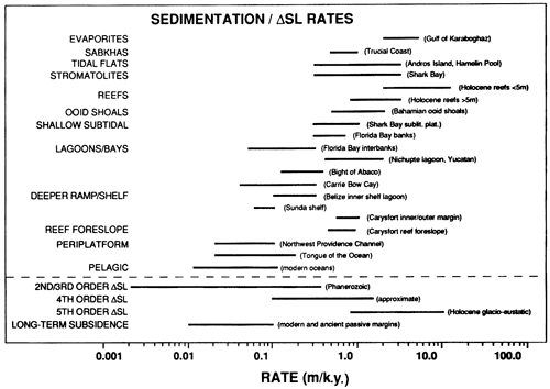
Estimations of sedimentation rates are based on the thickness of various Holocene units (which are underlain by the uppermost Pleistocene unconformity and capped by the modern depositional surface) divided by the time taken for the deposit to accumulate (fig. 1). Sedimentation rates are based on Holocene rates (Logan et al., 1974; Neumann and Land, 1975; Enos, 1977; Shinn et al., 1982; Bosence, 1989) with maximum values of deposition occurring in the shallow subtidal region, decreasing toward tidal flats and toward deeper water. Estimation of these rates is hampered by relative scarcity of well-dated cores from modern settings, by admixed layers of relict sediments that formed under more shallow-water settings during transgression, and in some cases by the presence of subaerial emergence surfaces of poorly known duration at the top of sections. These sedimentation rates are depositional rates that are averaged over the last few thousand years. They typically are much faster than long-term accumulation rates used in many models lacking high-frequency sea-level fluctuations. Long-term accumulation rates approximately match subsidence rates and include major periods of nondeposition, such as marine diastems, and many subaerial disconformities. The sedimentation rates also differ from short-term deposition rates measured over a few years, which are subject to highly variable depositional and erosional events related to storms (Hardie and Shinn, 1986).
Figure 1--Comparison of sedimentation rates of carbonate facies from various settings with rates of sea-level change and long-term 'subsidence. Compiled from various sources. Idea from Schlager (1981).
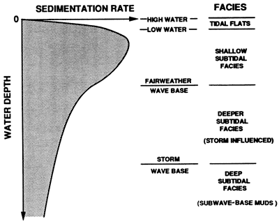
The sedimentation rates used in our model (fig. 2) commonly assume that maximum production and accumulation of carbonate occurs in the shallow subtidal zone and decreases with increasing water depth (Schlager, 1981). Depositional rates for selected water depths and facies are linearly interpolated for each 0.1 m (0.3 ft) of water depth. They can be adjusted to reflect postulated production rates of ancient marine communities and presence of hardgrounds or other indicators of slow deposition or nondeposition in the facies.
Figure 2--Sediment data file used in the model. The data used in most of the model runs were 0.3 m, 0.3 m/k.y.; 2 m, 0.4 m/k.y.; 5 m, 0.5 m/k.y.; 10 m, 0.3 m/k.y.; 20 m, 0.2 m/k.y.; 40 m, 0.1 m/k.y.; 300 m, 0.01 m/k.y. Tidal flat facies (not shown on longer runs), 0-2 m below high water; 2-5 m, shallow subtidal facies; 5-40 m, deeper subtidal facies; greater than 40 m, very deep subtidal facies.
Ultimately, sedimentation rates used in the model might also need to be decreased into interiors of rimmed platforms to reflect low circulation and restricted conditions and low productivity or precipitation. They also may need to be reduced in response to fine clastic poisoning resulting from increased turbidity.
The model generates a "rock type" for a specific water depth range (fig. 2). Because the model does not include energy regime but only water depth, it does not discriminate between muds, sands, and reefs for a given water depth. However, water depth ranges of "rock types" are chosen so that their boundaries coincide with likely water-depth limits of modern sedimentary facies types to ensure that the output is of maximum interpretive value. For example, the tidal range is used to bracket tidal flat facies. Shallow subtidal facies on the platform are extended from low tide down to some arbitrary depth and could include high-energy ooid or skeletal sands, reefs, or low-energy lagoonal muds. The depth of frequent storm reworking of the bottom is used to crudely separate storm -influenced facies on the deep ramp from deeper-water low-energy muds deposited below storm reworking.
The model incorporates subaerial erosion that is triggered after sea level drops below the sediment surface. Typical erosion rates for exposed carbonates range from 0.01 to 0.1 m/k.y. (0.03-0.3 ft/k.y.) (Trudgill, 1985). Carbonate sediment is eroded to sea level and is assumed to be dissolved and removed by ground water rather than redeposited. If the platform has been emergent for longer than a specified time (perhaps 10 k.y.), the sediment surface will be marked by a heavy line, indicating a disconformity.
Lag times are used in the model to simulate slow deposition or nondeposition following flooding of a previously emergent carbonate platform. Enos (1989) suggested that lag times actually reflect the time taken for flooding of the platform to create water depths favorable for formation of stable substrates, as opposed to wave-swept rock platforms. Because the time taken to reach this depth depends on relative sea-level rise rates, using the lag depth rather than the lag time might be better in modeling (Enos, 1989; Goldhammer et al., 1990). However, Enos and Perkins's (1979) data suggest that lag depths (and hence lag times) can vary significantly even in the same general area. For example, sea-level rise was tracked by tidal flats in the centers of some Florida Bay banks, whereas in other banks sedimentation lagged behind sea-level rise, resulting in an upward-deepening succession. Lag depths or times may increase as deposition moves onto the deeper seaward parts of carbonate platforms characterized by higher energy than platform interiors. For our model a uniform lag time, typically 1-5 k.y., is used across the platform, although any lag time (including zero) can be input by the user. Because both lag depths and lag times vary across platforms and even in the same area on a platform, it does not matter whether the lag time or the lag depth is used. Although lag times or depths are difficult to estimate, it seems unlikely from Holocene platforms that long lag times would occur on shallow-water platforms. Lag times have a major effect on the water depths generated on the platform, especially where sea-level fluctuations are of low amplitude. With short lag times, water depths remain shallow and asymmetric cycles are not generated.
Tidal ranges can be estimated from the thickness of the tidal flat lithofacies capping cycles, although these estimates are subject to considerable error. Tidal flat facies can be much thicker than the tidal range where they track sea-level rise or where two or more tidal flat facies are stacked and the contact between them is not recognized. Tidal flat facies may be much thinner than the tidal range where short-term sea-level oscillations are high and the flats develop during sea-level fall. Computer modeling helps to constrain likely tidal ranges (Koerschner and Read, 1989). Tidal range also can be estimated by comparing sedimentary structures in the caps with those occurring in modern micro- to macrotidal environments (Demicco, 1983). However, wide shallow shelves showing evidence of high tidal ranges may be more influenced by the effects of wind tides than by astronomic tides (Hagan and Logan, 1974; Hardie and Ginsburg, 1977).
The effects of compaction are not incorporated into the modeling program but are partially accounted for in the construction of stratigraphic cross sections. Decompaction corrections are critical for estimating original thicknesses of a sequence and depend on depth of burial, lithology, and effective stress. The percentage of increase in thickness can be estimated for various lithologies from the decompaction process performed during subsidence modeling. Based on the assumption of exponentially decreasing porosity with depth, decompacted thicknesses are calculated using the porosity versus depth curves of Bond and Kominz (1984). For predominantly carbonate lithologies buried under several kilometers of overburden, decompaction increases observed thicknesses by 10-25%. With increasing amounts of fine-grained siliciclastics, delithification increases observed thicknesses by 20-50%. Individual lithologies on stratigraphic cross sections created from observed thicknesses are differentially expanded by these estimates, and the decompacted cross sections are modeled.
The effects of compaction generally do not distort estimates of time, such as the duration of a sequence or average cycle period, unless one part of the succession compacts far differently from another. Decompacting the entire interval increases the subsidence rate, but, because the endpoints of the time interval are anchored, the duration of a component sequence or cycle remains the same. Because sequences and individual cycles decompact by the same proportion as the overall interval, for relatively uniform lithologies the duration does not change from the nondecompacted estimates.
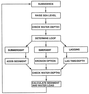
The model subdivides the platform to basin surface into 200 localities whose increment width is determined by the length of the profile. Antecedent topography is entered as a digitized profile, with the elevation of the platform surface set so that the required amount of accommodation space is ultimately generated (as a rule of thumb, total sediment thickness is roughly 2 or 3 times the space created by sea level and driving subsidence). The program (fig. 3) executes the calculations in user-specified time slices (usually 100-1,000 years). At any locality subsidence is computed, the position of sea level is calculated, and the water depth is determined. If the platform locality is emergent, no sediment is added and subsidence for the next time slice will be driving subsidence only. If the locality is submergent but undergoing lag, no sediment will be added and for the next time slice subsidence resulting from the new water load will be calculated for that locality and all adjacent localities affected by the load. If the platform is submergent and the lag time has elapsed, the sedimentation rate for that water depth is determined and the required amount of sediment is added. The water depth is then recalculated, and the isostatic subsidence component resulting from the water and sediment loads for that locality and all adjoining localities is computed. If the platform is emergent, the sediment surface can be eroded at a user-specified rate and a disconformity drawn at the top of the eroded sediment column. This procedure is done for all localities across the platform and then is repeated for subsequent time slices until the duration of the run has elapsed.
Figure 3--Flow chart illustrating steps involved in the two-dimensional modeling.
Most of the model runs presented here use a standard data file that is modified one parameter at a time to evaluate the effects of each parameter on the output. Slopes on the runs were set at 0.02 m/km (0.1 ft/mi) increasing to 0.1 m/km (0.5 ft/mi) toward the deep ramp. Tectonic subsidence may range from 0 at the cratonic hinge to 0.03 m/k.y. (0.1 ft/k.y.) at the distal portions of the platform (approximately one-third the average total subsidence rates of passive margins). The isostatic response time to loading was arbitrarily set at 5,000 years [equation for isostatic lag from Turcotte and Schubert (1982)]. The sea-level curve was generated using short-term periodicities of 19, 23, 41, and 100 k.y. Sedimentation rates used in the models are given in fig. 2.
Model runs (figs. 4-6) illustrate the combined effects of low-amplitude, high-frequency sea-level oscillations superimposed on third-order sea-level curves on a rotationally subsiding platform that responds elastically to water and sediment loading. The Milankovitch curve allows for the use of sedimentation rates that are relatively high and compatible with modern sedimentation rates measured over 103-104 years. However, the rates used in the model appear to be too high, judging by the large amount of progradation in the model output. If high-frequency signals are not superimposed on the third-order curve, sedimentation rates used in the modeling [usually up to 1.0 m/k.y. (3.3 ft/k.y.)] have to be constrained to low values that match long-term accumulation rates [usually 0.01-0.1 m/k.y. (0.03-0.3 ft/k.y.)], which commonly are 10 to 100 times less than depositional rates measured over several thousand years.
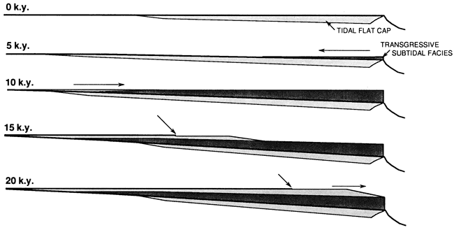
The models illustrate how an individual cycle or parasequence develops, using a symmetric 20-k.y. sea-level fluctuation and flooding an initially emergent platform (fig. 4). In the first 5 k.y. the platform undergoes regional flooding and a subtidal blanket forms, the leading edge of which onlaps the underlying disconformity. Because of the depositional lag following initial flooding, tidal flats are not developed on the transgressive surface. After 10 k.y. seaward-migrating tidal flats prograde over the landward margin of a blanket of subtidal sediments. After 15 k.y. the tidal flats extend across much of the platform, decreasing the area of the subtidal factory, and the inner portions begin to develop a disconformable surface. Finally, after 20 k.y. the platform is completely prograded by tidal flats, which are capped by a regional disconformity that passes seaward into a band of intertidal sediments. The carbonate factory is now limited to an extremely narrow band along the ramp margin, limiting the amount of carbonate production. Cycle development is renewed after the next rise in sea level in conjunction with rotational subsidence and loading by any sediments still accumulating in deeper water.
Figure 4--Computer simulation showing formation of a peritidal cycle on a previously emergent ramp, using 1 symmetric 20-k.y. sea-level fluctuation starting and ending at the lowstand of sea level. Time steps were calculated in 100-year increments. Resultant facies cross sections are shown at 5-k.y. intervals. Heavy line at start of run is disconformity at top of previous tidal flat capping platform. At 5 k.y., subtidal blanket onlaps platform in direction of arrow. At 10 k.y., tidal flat facies start to prograde in direction of arrow onto subtidal blanket. At 15 k.y., tidal flats extend halfway across platform and disconformity (leading edge marked by arrow) extends out over much of the inner platform. At 20 k.y., tidal flat facies extend completely across the platform and much of the platform surface is a disconformity (leading edge marked by arrow). Note that the depositional surface of the carbonate cycle generated is both aggrading and prograding.
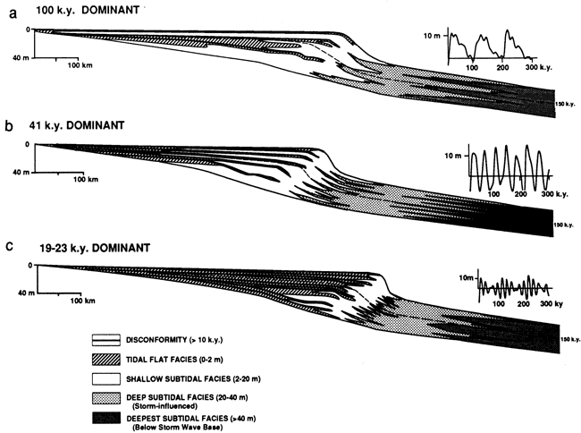
Effects of form of sea-level curve on peritidal cycle patterns
To examine the effects of the form of the sea-level curve on cycle formation, we used in the model runs several types of low-amplitude sea-level curves in which the 19-23-k.y., 41-k.y., or 100-k.y. signal was dominant for a duration of 300 k.y.
With a 100-k.y. signal of 10 m (33 ft) and the 41-k.y. and 19-23-k.y. signals suppressed to 2 m (7 ft), only fourth-order 100-k.y. cycles developed on the platform, resulting in a relatively simple platform stratigraphy (fig. 5a). Cycles commonly are several meters thick on the outer platform, thinning and pinching out onto the inner platform. Cycle-capping tidal flat facies range from thin to thick and are regional in extent.
With a dominant 41-k.y. signal of 10 m (33 ft) and the 100-k.y. and 19-23-k.y. signals suppressed to 2 m (7 ft), the cycle stratigraphy is more complex. Five to 7 cycles up to 5 m (16 ft) thick develop over much of the platform and thin landward (fig. 5b). Average cycle duration ranges from 40 to 60 k.y., depending on platform position. Inner peritidal platform cycles are mainly tidal flat facies, whereas outer peritidal platform cycles are dominated by subtidal lithofacies with thin tidal flat caps that are overlain by disconformities. On the subtidal portion of the synthetic platform, cycles are composed of lithofacies that reflect fluctuations of estimated fair-weather and storm wave base that move synchronously with sea-level oscillations. Seven subtidal cycles develop that reflect the 7 major sea-level events generated over 300 k.y. with the dominant 41-k.y. input signal.
With dominant 19-23-k.y. signals of 10 m (33 ft) and the 41-k.y. and 100-k.y. signals suppressed to 2 m (7 ft), platform stratigraphy is dominated by meter-scale cycles averaging between 30 and 40 k.y., depending on platform location (fig. 5c). The bulk of the peritidal platform is dominated by tidal flat facies, with thicker subtidal tongues limited to the outer subtidal platform. As pointed out by Goldhammer et al. (1987), meter-scale cycles approaching 20-k.y. periods must reflect dominant 20-k.y. sea-level fluctuations and suppressed 40-k.y. or 100-k.y. periods. Carbonate cycles in our model run are not deposited every 20 k.y. because of destructive interference among the 19-23-k.y., 41-k.y., and 100-k.y. sea-level signals.
Figure 5--Effects of form of Milankovitch sea level curve on types of cycles and their vertical and lateral relationships. Duration of run is 300 k.y. Sea-level curves are shown in insets. (a) Simulated stratigraphic cross section resulting from sea-level curve with a dominant 100-k.y. signal (10 m) and subordinate 41-k.y. and 19-k.y. and 23-k.y. signals (2 m). Platform stratigraphy dominated by 100-k.y. cycles. (b) Simulated stratigraphic cross section resulting from sea-level curve with a dominant 41-k.y. signal (10 m) and subordinate 100-k.y. and 19-23-k.y. signals (2 m). Platform stratigraphy shows common cycles with average 40-60-k.y. periods, depending on position on ramp. (c) Simulated stratigraphic cross section resulting from sea-level signal with dominant 19-k.y. and 23-k.y. signals (10 m) and subordinate 100-k.y. and 41-k.y. signals (2 m). Platform stratigraphy dominated by many high-frequency carbonate cycles.
Spencer and Demicco (1989) and Demicco et al. (this volume) have suggested that cycles can be made with relative sea-level fluctuations as little as a few centimeters related to subtle variations in eustasy or subsidence. However, to generate cycles under extremely low-amplitude sea-level oscillations, the user must limit sedimentation rates to a few centimeters per 1,000 years so that the sediment surface can track the long-term relative sea-level rise and fall. Unless these low sedimentation rates can be justified for all locations across a carbonate platform (including ooid shoals and ramp margin banks, which show modern rates many times this value), we doubt whether regional cycles can be formed in this way. With low-amplitude sea-level fluctuations such as these, the platforms would never be flooded to more than a few centimeters depth unless extremely long lag times (tens of thousands of years) were used to achieve the requisite lag water depths (Grotzinger, 1986; Koerschner and Read, 1989). For example, Goldhammer et al. (1990), on the basis of one-dimensional modeling, suggested that fourth-order autocycles could result from 2-m (7ft) lag depths interacting with a sea-level curve that lacks any fourth-order sea-level fluctuations. However, it would require 25-100 k.y. of subsidence to flood the platform to the required 2-m (7-ft) lag depth. This seems an excessive amount of time for nondeposition in less than 2 m (7 ft) of water across the entire platform. The autocycles of Goldhammer et al. (1990) do not show subaerial emergence; they merely reach sea level, in contrast to many actual peritidal cycles, which commonly show evidence of subaerial exposure and even vadose diagenesis related to eustatic sea-level fall (Goldhammer et al., 1987; Koerschner and Read, 1989).
Our two-dimensional modeling and that of Demicco et al. (this volume) show that extremely low amplitude sea-level fluctuations result in inner platform sections consisting totally of supratidal sediments, whereas seaward there are sections made up almost totally of intertidal sediments (fig. 6a). This facies distribution contrasts with actual cycles in the field, which consist of subtidal bases overlain by tidal and supratidal caps over most of the platform. Furthermore, with such low amplitudes we could not generate common deep ramp subtidal cycles that show a change from quiet deeper-water deposition upward into high-energy shallow subtidal deposition.
Given Holocene-based tidal flat sedimentation rates (fig. 1), thick tidal flat caps (fig. 6b) are developed with low-amplitude sea-level fluctuations of less than 10 m (33 ft) [100 k.y. of 5 m (16 ft), 41 k.y. of 3 m (10 ft), and 19- and 23-k.y. signals of 2 m (7 ft)]. With higher sea-level fluctuations of 20-40 m (66-131 ft), tidal flat caps are thin over most of the ramp and form significant local thickenings only on the landward edge of each cycle and on the seaward edges of tidal flat facies deposited during short-term lowstands (fig. 6c). Thick regional caps can be generated with these higher amplitudes only if tidal flat sedimentation rates are very high [>0.5 m/k.y. (>1.6 ft/k.y.)] or lag times are negligible or tidal range is high. With very high amplitude sea-level fluctuations [>100 m (>300 ft)], tidal flats are virtually absent and disconformities cap predominantly shallow subtidal facies at cycle tops over much of the platform and down the ramp slope (fig. 6d).
Figure 6--Effects of amplitude of high-frequency sea-level curve on simulated platform stratigraphy. Model runs of 300 k.y. duration. (a) Simulated platform stratigraphy resulting from extremely small fluctuations in sea level (less than 0.5 m). High-frequency cycles do not develop on the platform, even with low sedimentation rates of 0.1 m/k.y. The only way cycles could be generated under these conditions would be to have extremely long lag times of many tens of thousands of years that would allow the platform to subside to some lag depth, such as 2 m. (b) Simulated platform stratigraphy resulting from small Milankovitch fluctuations (100 k.y. equals 5 m, 41 k.y. equals 3 m, and 19-23 k.y. equals 2 m). Cycles tend to be layered and are dominated by tidal flat facies on platform. Aggraded platform surface at end of run has extremely low slope. (c) Simulated platform stratigraphy resulting from moderately high amplitude Milankovitch sea-level fluctuations (100 k.y. equals 20 m, 41 k.y. equals 12 m, and 19-23 k.y. equals 8 m). Small-scale cycles develop a shingled, lateral stacking pattern that complicates any layered stratigraphy. Note updip and downdip thickenings on landward and seaward extremities of tidal flat facies. Ramp surface evolves into a series of stepped depositional terraces. (d) Simulated platform stratigraphy resulting from high-amplitude Milankovitch sea-level fluctuations (100 k.y. equals 50 m, 41 k.y. equals 30 m, and 19-23 k.y. equals 20 m). Layered pattern of cycles is only poorly developed and is complicated by intense shingling of cycles, reflecting large-scale fluctuations of the strandline. Ramp surface retains considerable slope. Tidal flats virtually absent and cycles are thin and capped by disconformity.
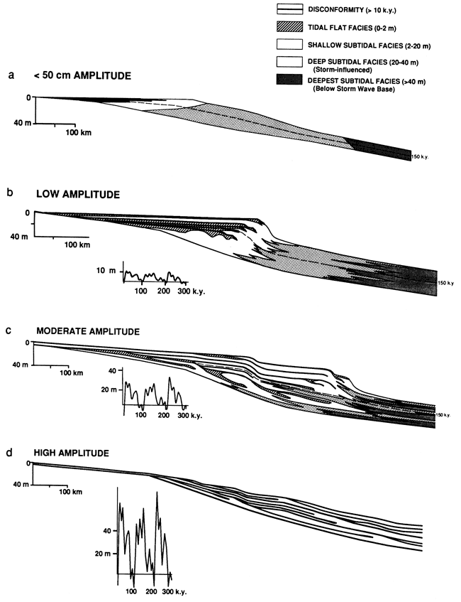
Increasing the amplitude of high-frequency sea-level fluctuations also has an important effect on the vertical and lateral stacking patterns of cycles. With small short-term fluctuations of sea level, cycles tend to be stacked in a layer-cake fashion across the platform (fig. 6b). However with an increase in amplitude, fifth-order cycles show both a vertical stacking and a shingled pattern of tidal flat units, reflecting small-scale rises and falls (20-40 k.y. duration) superimposed on the fourth-order transgressive-regressive pattern of the 100-k.y. fluctuations (figs. 6c,d). This shingling of tidal flat facies is most pronounced on the outer ramp, where many of the high-frequency cycles form small-scale offlapping units of limited regional extent. This shingling pattern is best developed with very high sea-level fluctuations [>100 m (>300 ft)] (fig. 6d). This results in a platform stratigraphy whose cycles would be extremely difficult to correlate from individual sections without numerous distinctive marker beds.
Deeper subtidal cycles that lack tidal flat caps are rarely developed in model runs with a low-amplitude curve with a 5-m (16-ft) 100-k.y., 3-m (10-ft) 41-k.y., and 2-m (7-ft) 19-23-k.y. signal, except in a narrow band on the ramp margin and a narrow band in deeper water (fig. 6b). In those areas showing some subtidal cyclicity, the intertonguing results in only two-component cycles, that is, shallow-water facies and slightly deeper facies on the upper slope or slightly deeper water facies and deep-water muds downslope. With these low amplitudes there is no intertonguing of all three facies.
Better intertonguing occurs with sea-level curves whose fluctuations exceed 10 m (30 ft), resulting in much broader bands with two-component cycles. However, three-component subtidal cycles still are not produced because the magnitude of the sea-level fluctuation is relatively small compared with the water depths separating the three component lithofacies (e.g., the water depths separating fairweather and substorm wave-base facies; fig. 2).
Successions containing well-developed three-component cycles are formed only where the sea-level fluctuations tend to exceed the depth between fairweather wave base and storm wave base (fig. 6c). Because this is a 30-m (100-ft) range for the sediment data file used, sea-level fluctuations would have had to exceed 30 m (100 ft). However, in protected intrashelf basins, where the depth to fairweather and storm wave base could be relatively shallow, perhaps as little as 15 m (49 ft) to storm wave base, sea-level fluctuations could be relatively small [say, 10 m (33 ft)] and still generate many three-component cycles. Both two- and three-component subtidal cycles are formed on the ramp margin and in deeper water with moderate-amplitude sea-level fluctuations (fig. 6c). This is commonly observed in the geologic record. Further seaward, two-component cycles composed of storm deposits that cap muds are typical. For moderate-amplitude sea-level fluctuations, the shallow-water caps on these deeper subtidal cycles generally do not become exposed by sea-level fall.
Model runs of 3 m.y. or more allow for the simulation of platform geometry and internal cyclic stratigraphy of third-order sequences and thus lead to a better understanding of the relations between superimposed third- to fifth-order sea-level oscillations, subsidence rates, sedimentation rates, antecedent topography, and development of systems tracts. The models (figs. 7a-c) clearly illustrate the relationship between the third-order sea-level curves and the resulting sequence stratigraphy in terms of location of ramp margin wedges (RMWs), transgressive systems tracts (TSTs), maximum flooding surfaces (MFSs), highstand systems tracts (HSTs), capping disconformities, and sequence -bounding unconformities.
Figure 7--Simulated platform stratigraphy containing two stacked sequences (1.5 m.y. durations) resulting from standard data file (see text and fig. 2). Duration of model run, 3 m.y. Time lines are 500-k.y. intervals. Because of the vertical exaggeration, the ramp margins appear steep but are in fact gently sloping. (a) Initial platform morphology and sea-level curve used to generate the cross sections. Systems tracts and sequence boundaries are shown on the sea-level curve. (b) Model run without erosion. RMW downlaps onto deeper-water facies and onlaps sequence boundary on ramp. TST cycles progressively onlap sequence boundary. MFS marked by furthest landward extension of deeper subtidal tongue onto ramp. Seaward, MFS marks turnaround from slight retrogradation of subtidal facies to aggradation. HST marked by widespread peritidal cycles. Base of second sequence shows marked onlap onto the sloping ramp surface (top of sequence 1). Platform stratigraphy contains numerous tidal flat capped cycles with well-developed subtidal bases that extend far onto platform. (c) Same conditions as in part b but with erosion of 0.05 m/k.y. This results in an increase in accommodation space because of erosional lowering of the ramp surface during emergence events. This allows more subtidal facies to accumulate and also thins or completely removes the tidal flat caps of cycles. The result is a platform stratigraphy dominated by subtidal facies and many disconformities. Erosion at sequence boundary 1 during long-term sea-level fall truncates cycles updip, erosionally removes the landward part of the maximum flooding surface, and erosionally thins the HST of sequence 1 to form a relatively flat surface of transgression. This results in deposition of relatively layered cycles that show only minor onlap above the sequence boundary. Note that, if the run had been continued so that long-term sea level continued to fall to the lowstand position, the HST of sequence 2 would become erosionally beveled and thinned until it resembled the HST of sequence 1.
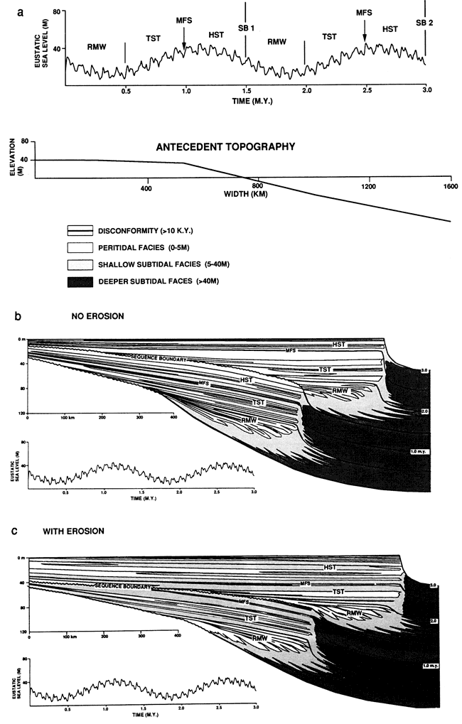
The model runs show variable development of RMWs during third-order lowstand, which in many cases coincides with the most seaward progradation of tidal flats of that sequence. Within the sequence maximum tidal flat progradation is not synchronous with the maximum sea-level fall rate, which marks the sequence boundary, but is associated with the RMW developed during the third-order sea-level lowstand. Ramp margin reefs or banks are likely to develop at this stage because the bulk of the platform is exposed, preventing inimical lagoonal waters from reaching ramp margin buildups, as occurs during periods when much of the platform is shallowly submerged. Ramp margin wedges appear to be best developed where ramp margin slopes are low (reflecting only gradual changes in sedimentation rates into deeper water) and where third-order and fifth-order sea-level fluctuations are tens of meters or more. The boundary between the RMW and the TST may be marked by a regional deepening.
Deposition of the TST starts with onset of the more rapid portion of the eustatic sea-level rise, which causes progressive onlap of cycles of the TST onto the emergent surface of the underlying sequence. The model runs illustrate that the TST has much thicker cycles than the HST, reflecting the greater accommodation space developed during long-term sea-level rise (Read and Goldhammer, 1988; Koerschner and Read, 1989; Goldhammer et al., 1990). The TST in two-dimensional carbonate models and in many actual sequences commonly is thick compared to clastic sequences, such as those described by Posamentier and Vail (1988) and Posamentier et al. (1988). This reflects how difficult it is to drown carbonate platforms (Schlager, 1981; Sarg, 1988). On carbonate ramps much sediment is produced in place across much of the ramp, commonly at a rate exceeding creation of long-term accommodation space. Thus drowning a carbonate ramp requires a major pulse of rapid subsidence (perhaps relatively rare in passive margins), a rapid short-term sea-level rise of many tens of meters, clastic poisoning of the carbonate factory, or a climate change causing a decrease in carbonate production. On clastic ramps sediment is introduced from the shoreline and consequently can be trapped in estuaries, so that net accumulation rates of clastic TSTs can be considerably less than long-term creation of accommodation space.
The model runs show that the turnaround between retrogradation or aggradation and progradation that denotes maximum flooding typically occurs slightly before the third-order highstand position of sea level and generally is clearly evident on the deeper ramp (figs. 7b,c). Commonly, it is not so clearly defined in the peritidal part of the ramp. However, in some model runs the MFS marks the base of a regional cycle with open marine facies that extends farthest onto the peritidal ramp. The landward extremities of the MFS can be removed by erosion at the sequence boundary (fig. 7c).
One-dimensional models and Fischer plots of sections from ramps can be misleading with regard to the relation of the MFS to the third-order sea-level curve. Goldhammer et al. (1990) suggest that for a flat-topped platform the MFS marks the time when the creation of accommodation space is at a maximum; thus they place its position at the time of maximum rise on the eustatic sea-level curve. This is not the case for ramps, because at the time of maximum eustatic rise only the seaward margins of ramps can be flooded; thus this cannot mark the MFS. Furthermore, creation of accommodation space at the time of maximum eustatic rise may not be at a maximum because only the outer part of the ramp and the basin are being flexurally loaded while the bulk of the inner ramp is only undergoing driving subsidence. Our two-dimensional model for ramps and published schematic model for clastic systems (Posamentier and Vail, 1988) suggest that the MFS occurs just before the third-order sea-level highstand, when the platform has undergone maximum regional flooding but creation of accommodation space is still high because of continued high rate of sea-level rise coupled with high flexural sediment and water loading across the whole ramp.
The two-dimensional model runs (figs. 7b,c) show that cycles of the HST tend to be thin and to show gradual offlap. However, this simple pattern is complicated by higher-frequency sea-level fluctuations that may contain small-scale fourth-order onlapping successions of cycles within the overall offlapping package. The HST cycles can show considerable diagenetic modification (dolomitization, leaching, brecciation) because of the increased duration of emergence of the caps, which results from the decreased accommodation space and numerous sea-level fluctuations that never flooded the ramp (Koerschner and Read, 1989; Goldhammer et al., 1990). Consequently, tidal flat caps of the HST may be brecciated or may develop as regoliths and be surfaced by well-developed disconformities.
The sequence-bounding unconformity on the inner ramp is initiated as the sea-level fall rate starts to exceed subsidence of the inner ramp (figs. 7b,c). When the maximum eustatic fall rate exceeds driving subsidence coupled with any load-induced flexural subsidence associated with ramp margin and deeper-water deposition, a regional unconformity develops. The duration of emergence is greatest on the inner ramp and decreases toward the outer ramp, where flexural load-induced subsidence tends to keep the ramp margin flooded, unless eustatic fall rates are high.
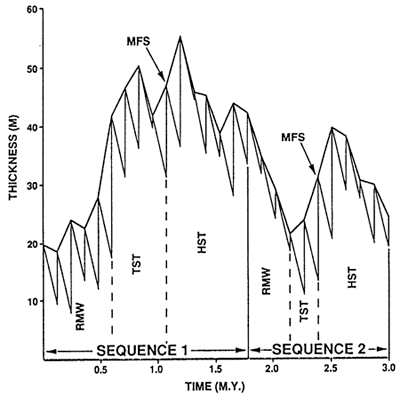
Erosion in the model has a significant effect on the relationship of the sequence boundary to underlying cycles (fig. 7c). Without erosion (fig. 7b), during long-term fall the cycles may show gradual offlap and feather out onto underlying cycles. With erosion, cycles of the HST are erosionally truncated along their updip parts (fig. 7c). With high erosion rates the bulk of the HST (sequence 1) is removed during sea-level fall. At the end of deposition of sequence 2, there is a well-developed HST, but this also would be stripped as sea level continued to fall to the lowstand position so that its final thickness would be similar to that of the HST of sequence 1. The TST of sequence 2 is deposited on a flat, erosionally beveled surface, causing the initial cycles of the TST to be far more extensive than if erosion did not occur. The models show that for short-term sequences (1-3-m.y. duration) that form under low-amplitude third-order sea-level fluctuations, high-frequency Milankovitch sea-level fluctuations can greatly complicate the sequence stratigraphy, making the boundaries between systems tracts difficult to define. If erosional surfaces are planar, sequence boundaries on the peritidal platform can be difficult to see in the field in limited lateral exposures. On the inner ramp where peritidal cycles commonly are disconformable, the unconformity marking the sequence boundary may be difficult to separate from any one of the cycle boundaries. On the outer peritidal ramp, where the duration of emergence associated with any sequence-bounding unconformity is likely to be of short duration, this problem is even more pronounced. Indirect evidence of a sequence boundary here might be stacking of thin cycles of the RMW above slightly thicker cycles of the HST (fig. 7c). Fischer plots can provide a simple method of recognizing the position of the RMW in single stratigraphic sections on the outer ramp. The RMW would presumably lie at the lowstand on the Fischer plot, whereas the sequence boundary would lie somewhere on the falling limb of the plot (fig. 8).
Figure 8--Fischer plot of simulated outer ramp section from fig. 7a. Plot grossly simulates two third-order sea-level cycles. However, magnitudes have 15-30% error compared with the input sea-level curves of 1.5-m.y. duration with 30-m amplitudes (see figs. 7a,b). Positions of the systems tract boundaries and sequence boundaries are shown and roughly correspond to their positions on the input sea-level curves. The major distortion in the plot relative to the original sea-level curve results from (1) the basal four cycles being subtidal and not dependent on accommodation space and (2) the change in load-induced subsidence from sequence 1 to sequence 2 resulting from basinward shift in the locus of deposition related to ramp progradation. Because the plot assumes linear uniform subsidence (calculated as average subsidence over 3 m.y.), the plot overestimates the sea-level fluctuation for sequence 1 and underestimates it for sequence 2.
The position of the sequence boundary also can be defined by the location of quartz sands at tops of cycles during third-order sea-level fall and lowstand, a feature shown by actual Fischer plots (Read and Goldhammer, 1988). Schematic sequence models (Posamentier and Vail, 1988) show a depositional break between the RMW and the underlying slope and basin facies of the HST. On ramps such a break might be due to the ramp being emergent during sequence boundary development and not supplying sediment to the adjacent deeper-water area. This can be simulated where off-platform sedimentation is a function of subtidal factory width. However, our two-dimensional model of carbonate ramps, whose sedimentation rates in these runs were not a function of factory width, show no such break; thus the sequence boundary at the ramp margin would have to be placed arbitrarily at the contact between the shallow to deep ramp facies and the underlying slope and deeper-water facies in individual sections.
Erosion of tops of individual small-scale cycles can produce cycle-capping disconformities as sea level periodically falls off the platform because of high-frequency sea-level oscillations (figs. 7b,c). If erosion rates are sufficiently high or if cycles are sufficiently long, tidal flat facies can be completely removed from the upper parts of cycles, leaving sequences dominated by subtidal facies punctuated by numerous erosional surfaces. Erosional removal of the upper parts of cycles may flatten the platform slopes, increase accommodation space, and allow for increased water depths during the ensuing transgression, allowing more open marine facies to develop on the platform compared to sections lacking erosional removal of strata.
Model runs suggest some of the controls that influence carbonate ramps. The large amount of progradation in the model runs appears to be too high, suggesting that the sedimentation rates used in the model may have been too high. Rotational subsidence of the ramp coupled with long duration of emergence of the platform during third-order sea-level fall has a major control on the slope of the surface of transgression. The faster the rotational subsidence and the longer the time of emergence, the steeper the slope of the surface of transgression.
A second control on ramp slopes is the amplitude of fifth-order sea levels. With amplitudes less than 10 m (30 ft), ramp slopes on the peritidal surface tend to aggrade to slopes of a centimeter or so per kilometer (figs. 6a,b). With increasing magnitude of sea-level fluctuations, the ramp surface tends to retain considerable slope, governed by the width of the platform and the magnitude of the fifth-order sea-level fluctuation (figs. 6c,d). This results from sea level migrating rapidly many times across the ramp, laying down relatively thin, seaward-dipping cycles. High-amplitude fifth-order fluctuations (fig. 6d) inhibit development of thick outer ramp margin sections characterized by high sedimentation rates, which would tend to flatten the slope. This is because water depths fluctuate rapidly with suppressed sedimentation rates in deep water and erosion in emergent areas. Consequently, little time is spent in shallow-water depositional settings where high sedimentation rates promote rapid shallowing of the ramp margin and flattening of the slope. This may account for the high slopes of many modern ramps, which were subjected to high-amplitude glacio-eustatic fluctuations of over 100 m (300 ft) during the Pleistocene.
Slopes on the ramp margin into deeper water are predominantly controlled by the difference in sedimentation rates on the shallow ramp versus those on the deeper ramp slope, a relationship probably determined by original depositional bathymetry. If sedimentation rates decrease only gradually into deeper water, where accumulation rates likely are a few centimeters per 1,000 years, slopes will remain ramplike. However, where sedimentation rates on the shallow ramp are far greater than those on the deeper ramp, the ramp margin slopes will rapidly steepen, tending toward development of a rimmed shelf.
Slopes on ramps may undergo subtle changes during a third-order cycle (figs. 7b,c). Slopes tend to be at a minimum during the third-order sea-level lowstand when the locus of sedimentation migrates rapidly out from the earlier ramp margin. Slopes increase during deposition of the TST because of increased accommodation space and low sedimentation rates in the now deeper basin.
The two-dimensional model allows evaluation of the use of Fischer plots to define systems tracts and magnitudes of third-order sea-level fluctuations (fig. 8). Fischer plots do not exactly represent the third-order sea-level fluctuation because they do not incorporate the effects of flexural loading and because they cannot assign time accurately to each cycle. Furthermore, Fischer plots give reasonable estimates of the sea-level change only where the full sea-level fluctuation is experienced by the specific stratigraphic section, typically on the outer ramp. On the shallow ramp the surface may be subjected to only the highstand part of the rise and fall; thus the plots tend to underestimate the magnitude of the third-order sea-level fluctuation. Fischer plots cannot be adequately tested using most one-dimensional models (Read and Goldhammer, 1988; Goldhammer et al., 1990) because these models neglect flexural loading of the ramp. Consequently, Fischer plots should be used with caution to define magnitudes of sea-level changes, with a clear understanding of their shortcomings. Sections used to estimate magnitude should be confined to the most seaward, cyclic peritidal locations. However, Fischer plots are extremely useful for defining approximate sea-level changes and for correlating systems tracts across peritidal platforms. In fact, they may provide the only way to correlate systems tracts on peritidal platforms using spaced stratigraphic sections where seismic data are lacking.
The two-dimensional model also is valuable for testing magnitudes of third-order sea-level rise and fall used in the models. If too small a third-order fluctuation is used, the sequence will be too thin and the sequences will tend to remain conformable far onto the platform. If too great a third-order rise and fall is used, the sequence will be too thick and, potentially, the highstand or regressive phase will be represented by a regional unconformity because sea level falls off the platform faster than driving subsidence. It should be pointed out that, in basins that continue to receive sediment during sea-level fall, continued sediment loading in deeper-water locations causes subsidence of the outer ramp to be considerably in excess of tectonic subsidence rates. Consequently it is difficult to generate unconformities along the outer ramp unless large sea-level fall rates are used.
Two-dimensional modeling that focuses on reproducing the meter-scale facies patterns within third-order sequences (1-10 m.y. duration) provides a rapid means of assessing likely controls on the development of meter-scale cycles and depositional sequences.
Computer programing was started by Sriram S. and carried to completion by Vincent Miranda, to whom we are especially grateful. We also thank Edwin Robinson and Cahit Çoruh for help with geophysical problems. We would like to thank reviewers Dave Lawrence, Cliff Frohlich, and Chris Kendall for their helpful comments. We also would like to thank Texaco, Chevron, Mobil, Marathon, and Arco for financial support of the Carbonate Research Laboratory at Virginia Tech. Typing was done by Belinda Pauley. Funding also was provided by the National Science Foundation under grant EAR 88-1779-05 to J. F. Read and by the Petroleum Research Foundation (American Chemical Society) under a grant to J. F. Read and D. A. Osleger.
Aigner, T., Doyle, M., Lawrence, D., Epting, M., and van Vliet, A., 1988, Quantitative modeling of carbonate platforms--some examples; in, Controls on Carbonate Platform and Basin Development, P. D. Crevello, J. L. Wilson, J. F. Sarg, and J. F. Read, eds.: Society of Economic Paleontologists and Mineralogists, Special Publication 44, p. 27-37
Anderson, R. Y., 1986, The varve microcosm--propagator of cyclic bedding: Paleoceanography, v. 1, p. 373-382
Arthur, M. A., Dean, W. E., Bottjer, D. J., and Scholle, P. A., 1984, Rhythmic bedding in Mesozoic-Cenozoic pelagic carbonate sequences--the primary and diagenetic origin of Milankovitch-like cycles; in, Milankovitch and Climate, A. L. Berger, J. Imbrie, J. Hays, G. Kukla, and B. Saltzman, eds.: D. Reidel, Dordrecht, Netherlands, p. 191-222
Bice, D., 1988, Synthetic stratigraphy of carbonate platform and basin systems: Geology, v. 16, p. 703-706
Bond, G. C., and Kominz, M. A., 1984, Construction of tectonic subsidence curves for the early Paleozoic miogeocline, southern Canadian Rocky Mountains--implications for subsidence mechanisms, age of breakup, and crustal thinning: Geological Society of America, Bulletin, v. 95, p. 155-173
Bond, G. C., Kominz, M. A., Grotzinger, J. P., and Steckler, M. S., 1989, Role of thermal subsidence, flexure, and eustasy in the evolution of early Paleozoic passive margin carbonate platforms; in, Controls on Carbonate Platform and Basin Development, P. D. Crevello, J. L. Wilson, J. F. Sarg, and J. F. Read, eds.: Society of Economic Paleontologists and Mineralogists, Special Publication 44, p. 39-61
Bosence, D. W. J., 1989, Biogenic carbonate production in Florida Bay: Bulletin of Marine Sciences, v. 44, p. 419-433
Bosence, D., and Waltham, D., 1990, Computer modeling the internal architecture of carbonate platforms: Geology, v. 18, p. 26-30
Burton, R., Kendall, C. G. St. C., and Lerche, I., 1987, Out of our depth--on the impossibility of fathoming eustatic sea level from the stratigraphic record: Earth Science Reviews, v. 24, p. 237-277
de Boer, P. L., and Wonders, A. A., 1984, Astronomically induced rhythmic bedding in Cretaceous pelagic sediments near Moria (Italy); in, Milankovitch and Climate, A. L. Berger, J. Imbrie, J. Hays, G. Kukla, and B. Saltzman, eds.: D. Reidel, Dordrecht, Netherlands, p. 177-190
Demicco, R. V., 1983, Wavy and lenticular-bedded carbonate ribbon rocks of the Upper Cambrian Conococheague limestone, central Appalachians: Journal of Sedimentary Petrology, v. 53, p. 1,121-1,132
Enos P., 1977, Holocene sediment accumulations of the south Florida shelf margin; in, Quaternary Sedimentation in South Florida, P. Enos and R. D. Perkins, eds.: Geological Society of America, Memoir 147, p. 1-130
Enos P., 1989, Lag time--is it simply storm-wave base?; in, Sedimentary Modeling--Computer Simulations of Depositional Systems, E. K. Franseen and W. L. Watney, eds.: Kansas Geological Survey, Subsurface Geology Series 12, p. 41-42
Enos, P., and Perkins, R. D., 1979, Evolution of Florida Bay from island stratigraphy: Geological Society of America, Bulletin, v. 90, p. 59-83
Fischer, A. G., 1964, The Lofer cyclothems of the Alpine Triassic; in, Symposium on Cyclic Sedimentation, D. F. Merriam, ed.: Kansas Geological Survey, Bulletin 169, p. 107-150 [available online]
Goldhammer, R. K., Dunn, P. A., and Hardie, L. A., 1987, High frequency glacio-eustatic sea-level oscillations with Milankovitch characteristics recorded in Middle Triassic platform carbonates in northern Italy: American Journal of Science, v. 287, p. 853892
Goldhammer, R. K., Dunn, P. A., and Hardie, L. A., 1990, Depositional cycles, composite sea-level changes, cycle stacking patterns, and the hierarchy of stratigraphic forcing--examples from Alpine Triassic platform carbonates: Geological Society of America, Bulletin, v. 102, p. 535-562
Greenlee, S. M., and Moore, T. C., 1988, Recognition and interpretation of depositional sequences and calculation of sea-level change from stratigraphic data---offshore New Jersey and Alabama Tertiary; in, Sea-Level Changes--An Integrated Approach, C. K. Wilgus, B. S. Hastings, C. G. St. C. Kendall, H. W. Posamentier, C. A. Ross, and J. C. Van Wagoner, eds.: Society of Economic Paleontologists and Mineralogists, Special Publication 42, p. 329-353
Grotzinger, J. P., 1986, Cyclicity and paleoenvironmental dynamics, Rocknest platform, northwest Canada: Geological Society of America, Bulletin, v. 97, p. 1,208-1,231
Hagan, G. M., and Logan, B. W., 1974, Development of carbonate banks and hypersaline basins, Shark Bay, Western Australia; in, Evolution and Diagenesis of Quaternary Carbonate Sequences, Shark Bay, Western Australia, B. W. Logan, ed.: American Association of Petroleum Geologists, Memoir 22, p. 61-139
Haq, B. U., Hardenbol, J., and Vail, P. R., 1987, Chronology of fluctuating sea levels since the Triassic: Science, v. 235, p. 1,156-1,167
Hardie, L. A., and Ginsburg, R. N., 1977, Layering--the origin and environmental significance of lamination and thin bedding: Johns Hopkins University Press, Baltimore, Maryland, p. 4276
Hardie, L. A., and Shinn, E. A., 1986, Carbonate depositional environments, modern and ancient--pt. 3, tidal flats: Colorado School of Mines Quarterly, v. 81, p. 1-74
Hays, J. D., Imbrie, J., and Shackleton, J. J., 1976, Variations in the Earth's orbit--pacemaker of the ice ages: Science, v. 194, p. 1,121-1,132
Herbert, T. D., and Fischer, A. G., 1986, Milankovitch climatic origin of mid-Cretaceous black shale rhythms in central Italy: Nature, v. 321, p. 739-743
Jeffreys, H., 1976, The earth: Cambridge University Press, Cambridge, England, 438 p.
Koerschner, W. F., and Read, J. F., 1989, Field and modeling studies of Cambrian carbonate cycles, Virginia Appalachians: Journal of Sedimentary Petrology, v. 59, p. 654-687
Kominz, M. A., and Bond, G. C., 1989, Are cyclic sediments periodic?; in, Sedimentary Modeling--Computer Simulations of Depositional Systems, E. K. Franseen and W. L. Watney, eds.: Kansas Geological Survey, Subsurface Geology Series 12, p. 35
Lawrence, D. T., Doyle, M., and Aigner, T., 1990, Stratigraphic simulation of sedimentary basins--concepts and calibration: American Association of Petroleum Geologists, Bulletin, v. 74, p. 273-295
Lerche, I., Dromgoole, E., Kendall, C. G. St. C., Walter, L. M., and Scaturo, D., 1988, Geometry of carbonate bodies--a quantitative investigation of factors influencing their evolution: Carbonates and Evaporites, v. 2, p. 15-42
Logan, B. W., Read, J. F., Hagan, G. M., Hoffman, P., Brown, R. G., Woods, P. J. and Gebelein, C. D., 1974, Evolution and diagenesis of Quaternary carbonate sequences, Shark Bay, Western Australia: American Association of Petroleum Geologists, Memoir 22, 358 p.
Moore, T. C., Loutit, T. S., and Greenlee, S. M., 1987, Estimating short-term changes in sea level: Paleoceanography, v. 2, p. 625-637
Neumann, A. C., and Land, L. S., 1975, Lime mud deposition and calcareous algae, Bight of Abaco, Bahamas--a budget: Journal of Sedimentary Petrology, v. 45, p. 763-786
Olsen, P. E., 1986, A 40-million-year lake record of early Mesozoic orbital climatic forcing: Science, v. 234, p. 842-848
Palmer, A. R., 1983, The decade of North American geology, 1983 geologic time scale: Geology, v. 11, p. 503-504
Posamentier, H. W., Jervey, M. T., and Vail, P. R., 1988, Eustatic controls on clastic deposition, I--conceptual framework; in, Sea-Level Changes--An Integrated Approach, C. K. Wilgus, B. S. Hastings, C. G. St. C. Kendall, H. W. Posamentier, C. A. Ross, and J. C. Van Wagoner, eds.: Society of Economic Paleontologists and Mineralogists, Special Publication 42, p. 109-124
Posamentier, H. W., and Vail, P. R., 1988, Eustatic controls on clastic deposition, II--sequence and systems tract models; in, Sea-Level Changes--An Integrated Approach, C. K. Wilgus, B. S. Hastings, C. G. St. C. Kendall, H. W. Posamentier, C. A. Ross, and J. C. Van Wagoner, eds.: Society of Economic Paleontologists and Mineralogists, Special Publication 42, p. 125-154
Read, J. F., and Goldhammer, R. K., 1988, Use of Fischer plots to define third-order sea level curves in peritidal cyclic carbonates, Early Ordovician, Appalachians: Geology, v. 16, p. 895-899
Sarg, J. F., 1988, Carbonate sequence stratigraphy; in, Sea-Level Changes--An Integrated Approach, C. K. Wilgus, B. S. Hastings, C. G. St. C. Kendall, H. W. Posamentier, C. A. Ross, and J. C. Van Wagoner, eds.: Society of Economic Paleontologists and Mineralogists, Special Publication 42, p. 156-181
Scaturo, D. M., Strobel, J. C., Kendall, C. G. St. C., Wendte, J. C., Biswas, G., Bezdek, J. C., and Cannon, R. C., 1989, Judy Creek, a case study for a two-dimensional sediment deposition simulation; in, Controls on Carbonate Platform and Basin Development, P. D. Crevello, J. L. Wilson, J. F. Sarg, and J. F. Read, eds.: Society of Economic Paleontologists and Mineralogists, Special Publication 44, p. 63-78
Schlager, W., 1981, The paradox of drowned reefs and carbonate platforms: Geological Society of America, Bulletin, v. 92, p. 197-211
Shinn, E. A., Hudson, J. H., Halley, R. B., Lidz, B., Robbin, D. M. and Macintyre, I. G., 1982, Geology and sediment accumulation rates---Carrie Bow Cay, Belize: Smithsonian Contributions to Marine Science, v. 12, p. 63-76
Spencer, R. J., and Demicco, R. V., 1989, Computer models of carbonate platform cycles driven by subsidence and eustasy: Geology, v. 17, p. 165-168
Steckler, M. S., and Watts, A. B., 1978, Subsidence of the Atlantictype continental margin off New York: Earth and Planetary Science Letters, v. 41, p. 1-13
Trudgill, S., 1985, Limestone geomorphology: London and New York, Longman, 196 p.
Turcotte, D. L., and Schubert, G., 1982, Geodynamics--applications of continuum physics to geological problems: John Wiley and Sons, New York, 450 p.
Watts, A. B., and Ryan, W. B. F., 1976, Flexure of the lithosphere and continental margin basins: Tectonophysics, v. 36, p. 25-44
Weedon, G. P., 1986, Hemipelagic shelf sedimentation and climatic cycles--the basal Jurassic (Blue Lias) of south Britain: Earth and Planetary Science Letters, v. 76, p. 321- 335
Kansas Geological Survey
Comments to webadmin@kgs.ku.edu
Web version April 26, 2010. Original publication date 1991.
URL=http://www.kgs.ku.edu/Publications/Bulletins/233/Read/index.html