Kansas Geological Survey, Bulletin 233, p. 463-472
by
Robert V. Demicco1, Ronald J. Spencer2, Brent B. Waters3, and Kelly C. Cloyd4
1 SUNY at Binghamton
2 University of Calgary
3 Ground Water Associates, Inc.
4 New York State Department of Environmental Conservation
The Middle-Upper Cambrian Waterfowl Formation of the southern Canadian Rocky Mountains comprises (1) subtidal shelf facies, (2) ooid-peloid shoal facies, (3) outer-shelf tidal flat facies, (4) inner-shelf tidal flat facies, and (5) siliciclastic playa-mudflat facies. These facies are arranged in a deepening to shallowing to deepening pattern, representing one complete third-order cycle and the beginning of another. The Basic program MAPS was modified to model the facies of the Waterfowl Formation. Two examples are given: (1) a high-amplitude, oscillatory relative sea-level regime; and (2) a low-amplitude, oscillatory relative sea-level regime. Both regimes produce facies similar to those composing the Waterfowl Formation.
An Acrobat PDF file containing the complete paper is available (880 kB).
In recent years ancient coastal deposits have come under increasing scrutiny as the sea-level gauges of the ancient oceans (Vail et al., 1977, 1984; Haq et al., 1987). Ancient peritidal carbonate deposits carry an especially detailed record of sea-level history in that they (1) contain a wealth of sedimentary features that allow detailed paleoenvironmental reconstructions and (2) are characterized by a hierarchy of depositional cycles. Low-frequency third-order (1-10 m.y. period) depositional cycles some hundreds to thousands of meters thick include higher-frequency fourth-order (0.1-1 m.y. period) and fifth-order (0.01-0.1 m.y. period) cycles. Third-order cycles in platform carbonates are the unconformity -bounded sequences of seismic and sequence stratigraphic analysis. Fourth-order and fifth-order cycles together make up the shallow ing-upward sequences of James (1984) and partial shallowing-upward sequences [e.g., punctuated aggradational cycles (PACs) (Goodwin and Anderson, 1985; Strasser, 1988)] and have generated many contributions to the literature [see Hardie and Shinn (1986)]. Differentiation of fourth- and fifth-order cycles is difficult [cf. Hardie and Shinn (1986, table 2, p. 66)] because of imprecision in dating. Rarely, however, fourth- and fifth-order cycles can be differentiated. Fischer (1964) noted systematic variations in thicknesses of meter-thick cycles in the Triassic Dachstein Limestone of the southern Alps, which he termed megacyclothems. Goldhammer et al. (1987) used spectral analysis to demonstrate decameter-thick fourth-order cycles with meter-thick fifth-order cycles in the Triassic Latemar Limestone of the Dolomites.
Despite intense study over the last 30 years, the origins of these different depositional cycle types is still not well understood. Numerous techniques are available for quantitative analyses of third-order, fourth-order, and fifth-order cycles in platform carbonate deposits. These include Fischer plots (Fischer, 1964; Goldhammer et al., 1987, 1990; Read and Goldhammer, 1988; Read, 1989), spectral analysis of cycle thicknesses (Goldhammer et al., 1987; Hinnov and Goldhammer, 1988), detailed backstripping calculations (Bond et al., 1989), and computer modeling (Spencer and Demicco, 1989; Koerschner and Read, 1989; Goldhammer et al., 1990; and other papers in this volume). In the last few years one-dimensional and two-dimensional computer models of cyclic carbonate deposition have been a welcome step toward quantitative assessment of the roles that eustasy, tectonic subsidence, and sediment production have in controlling the stratigraphic record. However, rarely in these studies are sedimentologic logs of measured stratigraphic sections compared with synthetic computer-generated stratigraphic sections [however, see Goldhammer et al. (1990)]. Nor are composite facies cross sections constructed from correlated measured sections compared with synthetic cross sections generated by computer models. In this article we use the Basic computer program MAPS (Demicco and Spencer, 1989) to model third-order cycles (depositional sequences) and their component fourth-order cycles in the Middle-Upper Cambrian Waterfowl Formation of the southern Canadian Rocky Mountains west of Calgary, Alberta. Waterfowl Formation depositional sequences are modeled using both eustasy- and subsidence-driven regimes of relative sea-level change.
The stratigraphy of the Middle and Upper Cambrian rocks in the Western Ranges, Eastern Ranges, Foothills, and adjacent plains in southeastern Alberta is shown in fig. 1. Formations of the Eastern Plains, Foothills, and Eastern Ranges form a westward-thickening wedge, up to 2.5 km (1.5 mi) thick, composed of shales and carbonates deposited in a variety of shallow subtidal and peritidal environments on a passive margin (Bond and Kominz, 1984). Equivalent formations of the Western Ranges are predominantly shales with minor carbonates; they represent off-platform deposits (Aitken, 1966b, 1971, 1978, 1989; McIlreath, 1977; Bond and Kominz, 1984). The Middle-Upper Cambrian Waterfowl Formation is exposed across the Eastern Ranges and Foothills in a series of eastward and northeastward verging thrust sheets (fig. 2). Figure 3 is a restored stratigraphic cross section of the Waterfowl Formation from the Red Deer River on the northeast to Marble Canyon on the southwest (Waters, 1986). The Waterfowl Formation has a restored outcrop width of 140 km (87 mi) and varies in thickness from 165 m (541 ft) to the west to 55 m (180 ft) at the Red Deer River. Further east, the Waterfowl Formation pinches out in the subsurface within 100 km (60 mi) of the mountain front.
Figure 1--Stratigraphy of Middle to Upper Cambrian deposits of the Rocky Mountains and adjacent plains in southwestern Alberta.
Figure 2--Major structural and depositional elements of the southem Canadian Rocky Mountains. Numbers indicate locations of measured sections used to construct the profile (A-A') of the Waterfowl Formation shown in fig. 3. Stippled area underlain by Cambrian off-shelf shales. Thrusts are Brazeau (Bz), McConnell (Mc), Rundle (Ru), Sulphur Mountain (Sm), Bourgeau (Bo), Sawback Lake (Sb), Johnston Creek (Jo), Pipestone (Pi), Simpson Pass (Si), Mons (Mo), Chatter Creek (Ca), and Purcell (Pu). [Figure modified after Bond and Kominz (1984, fig. 4, p. 160).]
The exact nature of the Middle and Upper Cambrian shelf to basinal transition is controversial. Aitken (1971, 1989) postulated that a narrow shelf margin (the "Kicking Horse Rim"), composed of dolomitic grainstones and boundstones, separates the Middle and Upper Cambrian platform deposits of the Eastern Ranges from their basinal equivalents in the Western Ranges. Ludvigsen (1989) challenged this view for the Middle Cambrian "Cathedral escarpment" based on paleontologic data. Figure 4 is a map and cross section of the platform to basin transition exposed on Mt. Whymper. Here, the outcrop of the Middle to Upper Cambrian Waterfowl Formation mapped as a rim facies by Aitken (1971) on the western slopes of Mt. Whymper [0.5 km (0.3 mi) west of section 1], is a massive crystalline dolomite cross-cut by dikes and pipes of dolomitic breccias with "zebra" textures. No talus breccias or carbonate debris flow or turbidite deposits were observed in the equivalent basinal Middle Chancellor shale less than 3 km (2 mi) away. These observations suggest that the Kicking Horse Rim may be, at least in part, a diagenetic rather than a depositional feature. Instead, the Middle-Upper Cambrian Waterfowl Formation most likely represents a carbonate ramp deepening into a shale-carbonate basin to the west.
The exposed portions of the Waterfowl Formation can be divided into five facies (fig. 3): (1) subtidal shelf facies, (2) ooid-peloid shoal facies, (3) outer-shelf tidal flat facies, (4) inner-shelf tidal flat facies, and (5) siliciclastic playa-mudflat facies. These are briefly described and interpreted in what follows; see Waters (1986, 1988) and Cloyd (1990) for further details.
Figure 3--Restored cross section of facies that compose the Middle-Upper Cambrian Waterfowl Formation in southwestern Alberta. Section locations given in fig. 2. Compare with figs. 8 and 9. See Waters (1986) for further details.
Figure 4--Stratigraphic and sedimentologic relationships of the Waterfowl Formation platform margin on Mt. Whymper (fig. 2, section 1) and equivalent upper middle Chancellor Formation shales across Marble Canyon in the Vermilion Pass area of Kootenay National Park, British Columbia.
The subtidal shelf facies is composed mainly of burrow-disrupted couplets of limestone grainstone layers up to 0.05 m (0.2 ft) thick that grade upward into dolomitic mudstone layers, also up to 0.05 m (0.2 ft) thick (fig. 5a). The limestone layers have sharp bases with load casts into the underlying dolostone and display planar to wavy lamination; they grade from coarse- sand- sized intraclasts and skeletal fragments to fine-grained peloidal grainstones before grading into the overlying dolomitic mudstone. The dolomite mudstone layers have parallel fine laminae. Whole trilobite fossils and Planolites feeding traces are common on dolostone bedding surfaces. In addition, vertical burrow tubes up to 10 mm (0.4 in.) in diameter filled with dolomitic mudstone may disrupt the grainstone layers and commonly produce a thoroughly mottled rock in which irregular, discontinuous grainstone lenses are surrounded by dolomitic mudstone (fig. 5b). Such complete burrow mottling is most common in western sections.
Figure 5--Rock types composing the Waterfowl Formation. (a) Couplets composed of limestone grainstone layers (dark) that grade up into dolomitic mudstone layers (light). Layering in this example is planar and continuous. Matchbook gives scale. (b) Burrow mottled limestone-dolostone couplets. Knife is approximately 75 mm long. (c) Planar-tabular, large-scale, cross-stratified grainstones. Ruler is approximately 0.3 in long. (d) Bedding plain view of flat domal stromatolites capping shale to grainstone cycles in ooid-peloidal shoal facies of section 7. (e) Mudcracked, planar-laminated mudstones. Scale bar is 20 mm long. (f) Crinkle-laminated, prism-cracked mudstones. Knife is approximately 75 mm long.
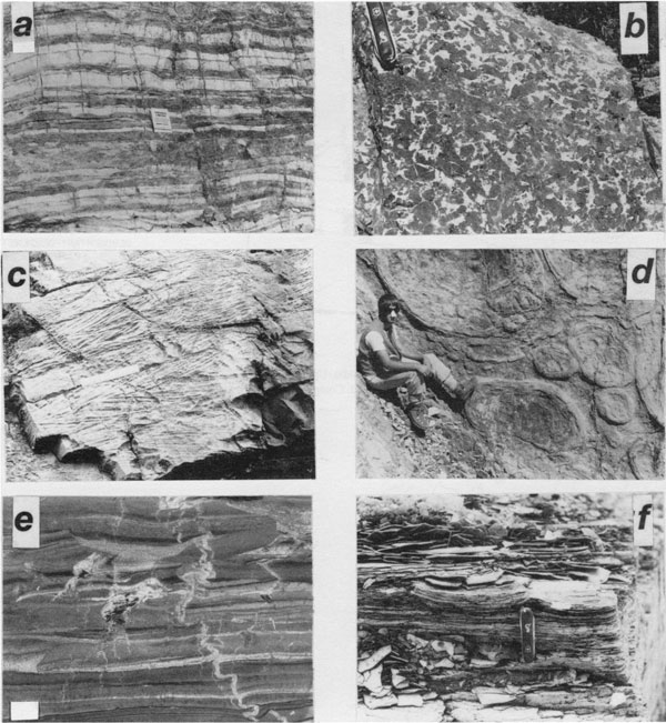
The subtidal shelf facies also contains stromatolite layers [up to 0.8 m (2.4 ft) thick], Renalcis-Girvanella thrombolites [up to 2 m (7 ft) in diameter], flat pebble lenses and layers up to 0.2 m (0.7 ft) thick, and massive peloidal-ooid grainstone layers up to 5 m (16 ft) thick (fig. 5c). A number of stromatolite layers, thrombolites, and grainstones apparently correlate across the various sections, whereas others do not (fig. 3). Particularly significant is a flat-pebble conglomerate with a dark shale matrix that occurs between 20 in and 30 m (66-98 ft) above the base of the formation; it is traceable laterally for more than 20 km (12 mi) (fig. 3).
Ooid-peloid shoal facies are restricted to eastern outcrops and occur at 16-31 m (52-101 ft) in section 8 and at 58-100 m (190-330 ft) in section 7 (fig. 3). In section 7 this facies has massive burrowed beds up to 2 m (7 ft) thick, sets of large-scale tabular and trough cross-strata up to 2 m (7 ft) thick, and Renalcis-Girvanella thrombolites up to 1 m (3 ft) thick. In section 8 this facies consists of 6 coarsening-upward cycles up to 3 m (10 ft) thick. Cycle bases are shales that contain halite hopper casts; they grade upward into large-scale cross-stratified ooid grainstone. The grainstones occur as crosscutting channels up to 3 m (10 ft) thick and tens of meters wide. The grainstones are in turn capped by flat domal stromatolites, 0.01 m (0.03 ft) thick and up to 3 m (10 ft) in diameter (fig. 5d). Cycles are traceable up to 20 km (12 mi) along strike.
Outer-shelf tidal flat facies form two westward-thickening wedges between sections 2 and 8 (fig. 3). This facies has well-defined fourth- or fifth-order cycles [1-10 m (3-33 ft) thick] that record a shallowing- upward environment (fig. 6). In general, cycles thicken westward. It is important to note that in the lower wedge of outer-shelf tidal flat facies the cycles thicken upward as well. In the upper wedge of outershelf tidal flat facies, the thinnest cycles are in the center of the wedge. Cycle bases in western outcrops predominantly comprise graded limestone grainstone-dolostone mudstone couplets [0.06 m (0.2 ft) thick] with lesser thrombolites, stromatolites, grainstones, and flat-pebble conglomerates. In eastern outcrops the cycle bases are large-scale cross-stratified peloidal grainstones. The central portions of all cycles consist of wavy and lenticular bedded "ribbon rocks" in which small-scale cross-stratified peloidal grainstones alternate with dolomitic mudstone drapes (Demicco, 1983). Waterfowl Formation ribbon rocks contain mudcracks and halite hopper casts. Cycles are capped by planar to crinkle laminated, prism-cracked mudstones (figs. 5e,f). A number of individual cycles are apparently correlative across sections 1 through 8 (fig. 6). However, one-for-one correlations of each cycle are not possible.
Figure 6--Correlation of rock types and thicknesses of five cycles composing the upper wedge of outer-shelf tidal flat facies at sections 5, 6, and 7 in the Waterfowl Formation. Section locations given in fig. 2. Sand divided into fine (f), medium (m), and coarse (c) grades.
Inner-shelf tidal flat facies are restricted to section 9 and the upper portions of section 8 (fig. 3). These complicated rocks consist of (1) multistory grainstone bodies with lateral accretion bedding, (2) discontinuous shallowing-upward cycles up to 1 m (3 ft) thick that pinch out laterally over hundreds of meters, and (3) thicker cycles that grade laterally into grainstone and stromatolitic mounds hundreds of meters across and up to 2 m (7 ft) high. Details of this facies can be found in the articles by Waters et al. (1989) and Cloyd et al. (1990).
Siliciclastic playa-mudflat facies are found in section 9. However, they are continuous for 100 km (60 mi) along strike on the McConnell thrust sheet. Aitken (1966a) and Aitken et al. (1984) interpreted this facies as the Sullivan Formation. However, detailed stratigraphic work along the McConnell thrust by Cloyd (1990) suggests that these are facies within the Waterfowl Formation. These facies comprise carbonate grainstone-siliciclastic mudstone cycles generally less than 1 m (3 ft) thick. The siliciclastic mudstones have deep, ptygmatically folded prism cracks and abundant halite hopper crystals.
We interpret the facies distribution within the Waterfowl Formation (fig. 3) to represent one complete transgressive-regressive third-order cycle or sequence and the partial record of a second (fig. 3). We interpret these cycles as third-order sequences because of their thickness [approximately 100 m (330 ft) for the complete sequence] and duration (the entire Waterfowl Formation represents approximately 3.2 m.y.; Bond and Kominz, 1984). The base of the formation represents a sequence boundary that separates the mainly terrestrial playa-marginal marine tidal flat deposits of the Arctomys Formation (Waters, 1986; Cloyd et al., 1990) from the marine Waterfowl Formation. These sequence boundaries are type 2 boundaries according to Haq et al.'s (1987) classification because subaerial unconformities are not generated. The lower wedge of the cycles represents a transgressive systems tract, developed during flooding of the platform. Each cycle is interpreted to record westward progradation of a tidal flat environment (James, 1984; Hardie and Shinn, 1986). Thickening of cycles upward within the lower wedge of outer-shelf cyclic facies is consistent with this interpretation [see Goldhammer et al. (1990)].
The graded limestone grainstone-dolostone mudstone couplets of the overlying subtidal shelf facies are interpreted as distal storm layers similar to modem graded sand-mud beds recovered from shallow siliciclastic and carbonate shelves (Howard and Reineck, 1981; Aigner, 1985). Thrombolites and stromatolites represent subtidal cyanobacterial bioherms, whereas the carbonate -matrix flat-pebble conglomerates represent proximal storm layers (Demicco, 1985; Waters, 1988). The laterally continuous, shale-matrix flat-pebble conglomerate in the overlying shelf facies is interpreted to represent the maximum flooding surface developed during the highstand of this relative sea-level rise (Haq et al., 1987).
We interpret the ooid-peloid shoal facies in section 8 as a barrier beach-saline lagoon complex developed where normal fairweather waves broke on the inshore portions of the ramp. The upward-desiccating cycles that developed landward of this barrier are interpreted as deposits of a siliciclastic playa to marginal marine mudflat environment (Cloyd, 1990). The subtidal shelf facies and bottom portion of the overlying outer shelf tidal flat cycles represent the highstand systems tract developed during relative sea-level fall. The exact position of the sequence boundary within the upper outer-shelf tidal flat cycles is ambiguous. We suggest that the thin cycle in the middle of the upper wedge of outer-shelf cyclic facies represents this sequence boundary [cf. Goldhammer et al. (1990)]. The overlying sequence includes the upper portions of the Waterfowl Formation and the overlying shaly Sullivan Formation. The cycles and subtidal shelf deposits represent the transgressive systems tract of this second relative sea-level rise. The maximum flooding surface of this sequence is above the top of the Waterfowl Formation.
The Basic program MAPS (Model Accumulation of Platform Sedimentation) simulates accumulation of carbonate platform sediments in two dimensions. Demicco and Spencer (1989) provide details of the program and the algorithm. Figure 7 is a flow chart for the MAPS program, which we have modified slightly for the current simulations. There are five categories of user-chosen variables as input to the program: (1) simulated length of time the program runs, (2) initial conditions across the platform, (3) controls on the relative sea level with time, (4) depth-dependent sediment production parameters, and (5) sediment distribution factors. The program executes 5 steps for each 10,000-year time increment.
Figure 7--Flow chart for the Basic program MAPS.
First, water depth is calculated for points spaced 1 km (0.6 mi) apart across the shelf. Second, a thickness of sediment is produced at each point based on the assigned depth-dependent sediment production rates. Third, sediment is transported according to input distribution factors. Sediment transported onshore builds up to the high tide and across the shelf until all transported sediment is deposited. In the fourth step the new sediment surface is plotted, and its position relative to sea level during that time increment is recorded. Finally, sea level is changed by an appropriate amount based on the input conditions for the next time increment. The program returns to the initial step until the specified simulated run length is reached. Thus the output consists of a two-dimensional representation of the height of the sediment surface across the shelf during each time step and the position of that surface relative to sea level.
Although our modeling considers a large number of variables, we do not consider isostasy or synsedimentary compaction. However, isostasy or synsedimentary compaction might be reasonably modeled by low-amplitude sea-level oscillations (Spencer and Demicco, 1989; see also later discussion). MAPS was modified by adding a hinge point to reproduce the facies of the Waterfowl Formation. In addition, the program was scaled to model several tens of meters of sedimentation at 10,000-year time steps. Facies patterns similar to those in the Waterfowl Formation can be simulated by MAPS in a variety of ways. Here we present two examples: one using high-amplitude relative sea-level oscillations and the other using low-amplitude relative sea-level oscillations.
Figure 8 simulates 3.33 m.y. of sedimentation produced by 3 superimposed relative sea-level changes: (1) a third-order sawtooth oscillation with a period of 1.6 m.y. and a height of 100 m (330 ft), (2) a fourth-order sinusoidal oscillation with a period of 160 k.y. and a height of 40 m (130 ft), and (3) a linear rise of 0.0255 m/k.y. (0.0837 ft/k.y.). The initial slope of the platform was 1:8,500 east of the hinge and 1:425 west of the hinge; the tidal range was 1 m (3 ft). Sediment production rates were 0.1 m/k.y. (0.3 ft/k.y.) from -70 m to -10 m (-230 to -30 ft) and 0.09 m/k.y. (0.2 ft/k.y.) from -10 m to 0 m (-30 to 0 ft). Sixty-five percent of the sediment accumulated in place, whereas 35% was transported shoreward, where it accumulated in prograding tidal flats.
Figure 8--(a) Computer simulation of Waterfowl Formation facies under high-amplitude sea-level oscillations: tidal range = 1 m. White = subtidal deposits (>-0.5 m below low tide level); light gray = shallow subtidal to intertidal deposits [-0.5 m below low tide level to mean sea level (MSL)]; dark gray = upper intertidal deposits (MSL to high tide level) or subaerial exposure surfaces. Gap in diagram is approximately 50 km. (b) Simplified cyclostratigraphy of part a at the same scale. Cycles generated during 21 fourth-order sea-level oscillations numbered and stippled. Subtidal areas unadorned. (c) Relative sea-level curve used to generate parts a and b. Duration is 3.7 m.y. Lower dotted line is original relative elevation of western shelf edge; middle dotted line is original relative elevation of hinge line; upper dotted line is original relative elevation of eastern shelf edge.
Under these conditions modified MAPS produces two wedges of tidal flat cycles separated by subtidal deposits west of the hinge line. Subtidal deposits everywhere overlie the upper wedge of tidal flat deposits. Each 160-k.y. fourth-order oscillation produced a prograding tidal flat deposit (numbered in fig. 8b). Cycles 1-5 and 11-15 were generated on the falling portions of third-order oscillations. Each tidal flat prograded during falling sea level [i.e., "descending progradation" (Hardie and Shinn, 1986, fig. 77, p. 64)]. Cycles 6-10 and 16-21 were generated on the rising portions of third-order oscillations. Thick subtidal deposits were produced on the western portions of platforms during these third-order rises. However, the prograding tidal flats accumulated under conditions of descending progradation. It is important to note that in this model initial sedimentation (model startup) takes place on a third-order fall. Thus cycles 1-5 here belong to the underlying Arctomys Formation, with cycles 610 representing the initial tidal flat cycles of the Waterfowl Formation. We have modeled 5 cycles in this lower transgressive systems tract, whereas there are 5-10 cycles measured in the field. However, changing the sea-level oscillation period would allow us to match any number between 5 and 10.
Figure 9 simulates 3.7 m.y. of sedimentation produced by 3 superimposed relative sea-level changes: (1) a third-order sawtooth oscillation with a period of 1. 8 m.y. and a height of 5 m (16 ft); (2) a fourth-order sinusoidal oscillation with a period of 200 k.y. and a height of 1 m (3 ft); and (3) a linear rise varying across the platform from 0.043 m/k.y. (0. 14 ft/k.y.) at the western edge to 0.018 m/k.y. (0.059 ft/k.y.) at the hinge to 0.015 m/k.y. (0.049 ft/k.y.) at the eastern edge. In addition, during the last 1 m.y., linear relative sea-level rise was increased to 0.048 m/k.y. (0. 16 ft/k.y.) at the western edge of the platform. The platform was flat at the start of the simulation; the tidal range was 1 m (3 ft). Sediment production rates were 0.06 m/k.y. (0.2 ft/k.y.) from -12 in to -3 m (-39 to -10 ft) and 0.04 m/k.y. (0.13 ft/k.y.) from -3 m to 0 m (-10 to 0 ft). Seventy percent of the sediment accumulated in place, whereas 30% was transported shoreward, where it accumulated in prograding tidal flats.
Figure 9--(a) Computer simulation of Waterfowl Formation facies under low-amplitude sea-level oscillations: tidal range = 1 in. White = subtidal deposits (>-0.5 m below low tide level); light gray = shallow subtidal to intertidal deposits (-0.5 in below low tide level to MSL); dark gray = upper intertidal deposits (MSL to high tide level) or subaerial exposure surfaces. Gap in diagram is approximately 50 km. (b) Relative sea-level curve used to generate part a. Duration is 3.33 m.y. Upper line is relative sea level at western shelf edge; middle line is relative sea level at hinge line; lower line is relative sea level at eastern shelf edge.
Under these conditions tidal flats can prograde across the platform during third-order sea-level falls. However, during third-order rises, tidal flats can prograde only about halfway across the shelf, and a wedge of subtidal deposits is produced in western portions. The increased subsidence at the end of the simulation results in drowning and thinning of the westward portion of the shelf, matching the transition of the Waterfowl Formation into the deep-water shales of the overlying Sullivan Formation.
Both synthetic cross sections (figs. 8 and 9) compare reasonably well with the reconstructed sedimentary facies of the Waterfowl Formation (fig. 3). These simulations demonstrate that similar facies patterns can be produced on carbonate shelves using relative sea-level oscillations that vary over several orders of magnitude. We deliberately chose two disparate sets of input variables to produce the two models, which vary only slightly from each other or from the field data. However, all the variables are well within the ranges suggested by the scant available data [cf. Hardie and Shinn (1986) and Spencer and Demicco (1989)]. Furthermore, these simulations are only two possible end members, with a variety of intermediate solutions also possible. Forty-meter (130-ft) amplitude sea-level oscillations modeled in fig. 8 are in the range of Pleistocene glacio-eustatic fluctuations. In contrast, the combination of relative sea-level oscillations modeled in fig. 9 yields net long-term relative rates of sea-level changes from 0.03 to 0.05 m/k.y. (0.1-0. 16 ft/k.y.). Such variations might reasonably model varying subsidence rates, isostasy, or compaction [see Spencer and Demicco (1989)].
It is important to note that variations in other modeling parameters can generate similar facies patterns. Variations in oscillation period can also be used to simulate variable subsidence and can produce similar facies patterns. Likewise, changes in sediment production rates or changes in sediment transport parameters also can produce the observed facies patterns. Such changes model climatic changes, circulation pattern shifts, and transport pathway variation (autocyclicity). It is unlikely that any unique cycle-forcing mechanism can be demonstrated through computer modeling because of the many independent variables that even simplistic models contain.
This article is based in part on an M.Sc. thesis by Waters, at the University of Calgary, and on a Ph.D. dissertation by Cloyd at SUNY, Binghamton. We acknowledge Parks Canada for permission to work in Banff, Kootenay, and Yoho national parks. Spencer received financial support from the Natural Sciences and Engineering Research Council of Canada. Demicco was supported by the National Science Foundation under grant EAR8511001. R. K. Goldhammer and J. F. Read reviewed the manuscript.
Aigner, T., 1985, Storm depositional systems--dynamic stratigraphy in modem and ancient shallow-marine sequences: Lecture Notes in Earth Sciences 3, Springer-Verlag, New York, 174 p.
Aitken, J. D., 1966a, Cambrian sections in the easternmost southern Rocky Mountains and the adjacent subsurface, Alberta: Geological Survey of Canada, Paper 66-23, 34 p.
Aitken, J. D., 1966b, Middle Cambrian to Middle Ordovician cyclic sedimentation, southern Canadian Rocky Mountains of Alberta: Bulletin of Canadian Petroleum Geology, v. 14, p. 405-442
Aitken, J. D., 1971, Control of lower Paleozoic sedimentary facies by the Kicking Horse Rim, southern Rocky Mountains, Canada: Bulletin of Canadian Petroleum Geology, v. 19, p. 557-569
Aitken, J. D., 1978, Revised models for depositional grand cycles, Cambrian of the southern Rocky Mountains, Canada: Bulletin of Canadian Petroleum Geology, v. 26, p. 515-542
Aitken, J. D., 1989, Birth, growth, and death of the Middle Cathedral carbonate lithosome, southern Rocky Mountains: Bulletin of Canadian Petroleum Geology, v. 37, p. 316-333
Aitken, J. D., Chappell, F., and Tippett, C. R., 1984, Unconformities and subcrop relationships: Canadian Society of Exploration Geologists Update '84, Field Trip Guidebook A2, Canadian Society of Petroleum Geology, 22 p.
Bond, G. C., and Kominz, M. A., 1984, Construction of tectonic subsidence curves for the early Paleozoic miogeocline, southern Canadian Rocky Mountains--implications for subsidence mechanisms, age of breakup, and crustal thinning: Geological Society of America, Bulletin, v. 95, p. 155-173
Bond, G. C., Kominz, M. A., Streckler, M. S., and Grotzinger, J. P., 1989, Role of thermal subsidence, flexure, and eustasy in the evolution of early Paleozoic passive-margin carbonate platforms; in, Controls on Carbonate Platform and Basin Development, P. D. Crevello, J. L. Wilson, J. F. Sarg, and J. F. Read, eds.: Society of Economic Paleontologists and Mineralogists, Special Publication 44, p. 39-61
Cloyd, K. C., 1990, Cyclic sedimentary sequences of the Middle-Upper Cambrian Waterfowl Formation along the McConnell thrust, western Alberta: Ph.D. dissertation, State University of New York, Binghamton, 156 p.
Cloyd, K. C., Demicco, R. V., and Spencer, R. J., 1990, Tidal channel, levee, and crevasse-splay deposits from a Cambrian tidal channel system--a new mechanism to produce shallowing-upwards sequences: Journal of Sedimentary Petrology, v. 60, p. 73-83
Demicco, R. V., 1983, Wavy and lenticular-bedded carbonate ribbon rocks of the Upper Cambrian Conococheague Limestone, central Appalachians: Journal of Sedimentary Petrology, v. 53, p. 1, 121-1,132
Demicco, R. V., 1985, Platform and off-platform carbonates of the Upper Cambrian of western Maryland: Sedimentology, v. 32, p. 1-22
Demicco, R. V., and Spencer, R. J., 1989, MAPS--a Basic program to model accumulation of platform sediments: Computers & Geosciences, v. 15, p. 95-105
Fischer, A. G., 1964, The Lofer cyclothems of the Alpine Triassic; in, Symposium on Cyclic Sedimentation, D. F. Merriam, ed.: Kansas Geological Survey, Bulletin 169, v. 1, p. 107-149 [available online]
Goldhammer, R. K., Dunn, P. A., and Hardie, L. A., 1987, High-frequency glacio-eustatic sea-level oscillations with Milankovitch characteristics recorded in Middle Triassic platform carbonates in northern Italy: American Journal of Science, v. 287, p. 853-892
Goldhammer, R. K., Dunn, P. A., and Hardie, L. A., 1990, Depositional cycles, composite sea-level changes, cycle stacking patterns, and the hierarchy of stratigraphic forcing--examples from platform carbonates of the Alpine Triassic: Geological Society of America, Bulletin, v. 102, p. 535-562
Goodwin, P. W., and Anderson, E. J., 1985, Punctuated aggradational cycles-a general model of episodic stratigraphic accumulation: Journal of Geology, v. 93, p. 515-534
Haq, B. U., Hardenbol, J., and Vail, P. R., 1987, Chronology of fluctuating sea levels since the Triassic: Science, v. 235, p. 1,156-1,166
Hardie, L. A., and Shinn, E. A., 1986, Carbonate depositional environments, modem and ancient--pt. 3, tidal flats: Colorado School of Mines Quarterly, v. 81, p. 1-74
Hinnov, L. A., and Goldhammer, R. K., 1988, The identification of Milankovitch signals in M. Triassic platform carbonates cycles using a super-resolution spectral technique (abs.): American Association of Petroleum Geologists, Bulletin, v. 72, p. 197
Howard, J. D., and Reineck, H. E., 1981, Depositional facies of high-energy beach-to-offshore sequence--comparison with low-energy sequence: American Association of Petroleum Geologists, Bulletin, v. 65, p. 807-830
James, N. P., 1984, Shallowing-upward sequences in carbonates; in, Facies Models, R. G. Walker, ed.: Geological Association of Canada, Reprint Series 2, p. 213-229
Koerschner, W. F., III, and Read, J. F., 1989, Field and modeling studies of Cambrian carbonate cycles, Virginia Appalachians: Journal of Sedimentary Petrology, v. 59, p. 654-687
Ludvigsen, R., 1989, The Burgess Shale--not in the shadow of the Cathedral escarpment: Geoscience Canada, v. 16, p. 51-59
McIlreath, I. A., 1977, Stratigraphic and sedimentary relationships at the western edge of the Middle Cambrian carbonate facies belt, Field, British Columbia: Ph.D. dissertation, University of Calgary, Calgary, Canada, 269 p.
Read, J. F., 1989, Modeling of carbonate cycles; in, Carbonate Sedimentology and Petrology, P.A. Scholle, N. P. James, and J. F. Read, eds.: American Geophysical Union, Short Course in Geology 4, p. 101-110
Read, J. F., and Goldhammer, R. K., 1988, Use of Fischer plots to define third-order sea-level curves in Ordovician peritidal cyclic carbonates, Appalachians: Geology, v. 16, p. 895-899
Spencer, R. J., and Demicco, R. V., 1989, Computer models of carbonate platform cycles driven by subsidence and eustasy: Geology, v. 17, p. 165-168
Strasser, A., 1988, Shallowing-upward sequences in Purbeckian peritidal carbonates (lowermost Cretaceous, Swiss and French Jura Mountains): Sedimentology, v. 35, p. 369-383
Vail, P. R., Hardenbol, J., and Todd, R. G., 1984, Jurassic unconformities, chronostratigraphy, and sea-level changes from seismic stratigraphy and biostratigraphy; in, Interregional Unconformities and Hydrocarbon Accumulation, J. S. Schlee, ed.: American Association of Petroleum Geologists, Memoir 36, p. 129-144
Vail, P. R., Mitchum, R. M., Jr., Todd, R. G., Widimier, J. M., Thompson, S., III, Sangree, J. B., Bubb, J. N., and Hateilid, W. G., 1977, Seismic stratigraphy and global changes of sea level; in, Seismic Stratigraphy--Applications to Hydrocarbon Exploration, C. E. Payton, ed.: American Association of Petroleum Geologists, Memoir 26, p. 49-212
Waters, B. B., 1986, Sedimentology and paleogeography of the Upper Cambrian Waterfowl Formation, southern Canadian Rockies: M.Sc. thesis, University of Calgary, Calgary, Canada, 216 p.
Waters, B. B., 1988 Upper Cambrian Renalcis/Girvanella framestone mounds, Alberta: Canadian Society of Petroleum Geologists, Memoir 13, p. 165-169
Waters, B. B., Spencer, R. J., and Demicco, R. V., 1989, Three-dimensional architecture of shallowing-upward carbonate cycles--Middle and Upper Cambrian Waterfowl Formation, Canmore, Alberta: Bulletin of Canadian Petroleum Geology, v. 37,p.198-209
Kansas Geological Survey
Comments to webadmin@kgs.ku.edu
Web version April 23, 2010. Original publication date 1991.
URL=http://www.kgs.ku.edu/Publications/Bulletins/233/Demicco/index.html