Original published in D. W. Steeples, ed., 1989, Geophysics in Kansas: Kansas Geological Survey, Bulletin 226, pp. 245-256

A case history of petroleum exploration in the southern Forest City basin using gravity and magnetic surveys

by Tom W. Stander

James L. Grant and Associates, Inc., Englewood, Colorado
The article is also available as an Acrobat PDF file.

Abstract

Three geophysical surveys were conducted in Johnson and Douglas counties in Kansas. The first two projects were gravity surveys each covering nearly 50 mi² (130 km²). In all three surveys, readings of the gravity or magnetic fields were taken along county roads at 1/4-mi (.4-km) intervals. Normal data reductions and corrections were applied to the data. The data were displayed as contoured Bouguer gravity maps and a diurnal tide-corrected magnetic map. The Bouguer gravity maps indicated gravity anomalies with 0.20-1.20 mgal closures. Many of the closures were elliptical with their long axes paralleling local structural trends. Some of the gravity anomalies corresponded to known oil and gas fields. In particular, the Gardner oil dome near Gardner, Kansas, is associated with a 0.80-mgal gravity anomaly. The magnetic map indicated closures of 60-80 gammas. Some of the magnetic data corresponded well with the gravity data. Like the gravity data, some of the magnetic anomalies corresponded to known oil and gas fields. Several wildcat wells were drilled on or near gravity or magnetic highs. The first notable find was the discovery well of the Little Wakarusa Creek oil field. Oil is now being produced from 14 wells in this field from a 15-ft (4.5-m)-thick Cherokee sandstone at a depth of about 700 ft (210 m). The oil field is located in southeastern Douglas County nearly 5 mi (8 km) south of Eudora, Kansas. Initial flush productions varied between 10 and 40 bbls of oil per day. The magnetic and gravity data were interpreted to be related to deep basement structures. The deeper structures (.5-3 mi [.8-4.8 km] in depth) influence near-surface structures in the Cherokee Group of Pennsylvanian rocks. The structures provided trapping mechanisms for hydrocarbon accumulation in the Cherokee sandstones.

Introduction

Oil and gas production in the southern Forest City basin has occurred since the first oil well was discovered by Dr. G. W. Brown near Paola in 1860 (Haworth, 1908). Production today is largely from shallow stripper wells producing from Pennsylvanian Cherokee sandstones.

Even though eastern Kansas is considered a mature exploration area, large undrilled areas still exist. The vast majority of wells in the southern and eastern parts of the basin penetrated only into the Pennsylvanian section. Deeper potential pay zones such as the Mississippian, Hunton, Viola, Simpson, and Arbuckle formations have not been drilled and tested adequately.

Relatively low-cost gravity and magnetic surveys were conducted in the southern portion of the Forest City basin as a method of identifying drilling sites in formerly undrilled areas.

Area

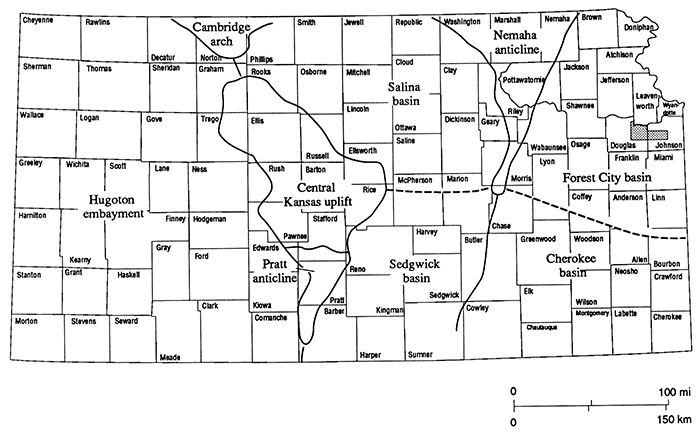
The three areas of the survey are in western Johnson and southeastern Douglas counties in eastern Kansas (fig. 1). The first gravity study area was a 4 x 12-mi grid (6.4 x 19.2-km; fig. 3) located in west-central Johnson County. The project area included the Gardner oil pool and parts of the Gardner South oil, Olathe gas, and Prairie Center gas pools. This gravity map is labeled Simple Bouguer map northwest of Gardner, Kansas.

Figure 1--Geophysical surveys located within the shaded area in Douglas and Johnson counties, Kansas.

The second gravity area was located in the southeastern portion of Douglas County. The 4 x 10-mi (6.4 x 16-km) grid includes sections in T. 14 S., R. 19, 20, and 21 E. This area (fig. 4) is labeled Simple Bouguer gravity map near Vinland, Kansas, and is nearly centered around the small town of Vinland.

The third area covers 132 mi² (343 km²) in east-central Douglas County. Both gravity and magnetic data were collected over the roughly 9 x 13-mi (14 x 21-km)grid. The city of Lawrence is located in the northwest corner of this map, known as the Southeast Lawrence gravity and magnetics map (figs. 5-7).

Geology

The exposed surface rocks of both Douglas and Johnson counties are of Pennsylvanian age belonging to the Shawnee, Douglas, Pedee, Lansing, and Kansas City groups. Portions of the northern parts of the counties are overlain by glacial drift.

The subsurface sediments are from Pennsylvanian to Cambrian age (fig. 2). The Pennsylvanian consists of 350 ft (105 m) of Lansing and Kansas City. The thickness of the Pleasanton-Marmaton-Cherokee section ranges from 700 to 1,000 ft (210-300 m).

Figure 2--Kansas reservoir rocks; after Moore et al. (1951), Hilpman (1958), and Merriam and Goebel (1968).

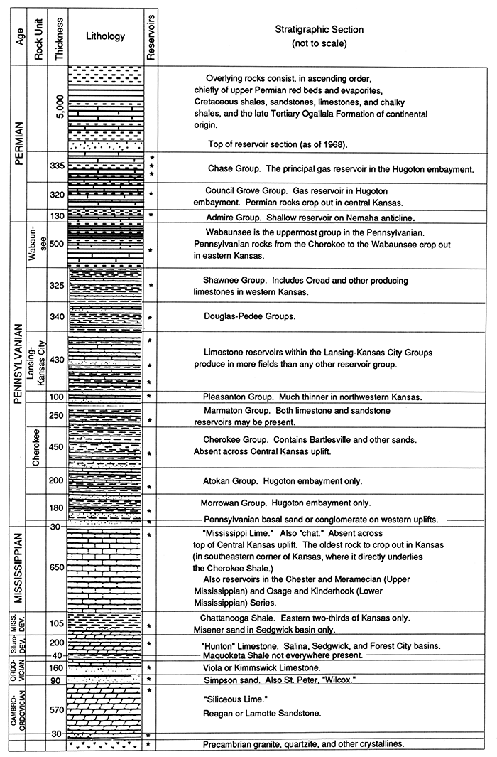
The Mississippian-age rocks range from 250 to 450 ft (75-135 m) thick and include the Spergen, Warsaw, Burlington, Sedalia, and Chouteau formations. The Chattanooga Shale ranges in thickness from less than 50 to as much as 100 ft (15-30 m).

Devonian rocks vary from 70 ft (21 m) thick in T. 12 S., R. 19 E., in Douglas County to 15 ft (4.5 m) thick in T. 14 S., R. 22 E. in Johnson County.

Silurian rocks, the Maquoketa Shale, and part of the Viola Limestone were removed by erosion from both counties before the deposition of the Devonian sediments. The Viola Limestone varies from 24 to 115 ft (7.2-34.5 m) thick. The Platts ville Shale ranges from 10 to 30 ft (3-9 m) thick. The St. Peter Sandstone ranges from 50 to 100 ft (15-30 m) in thickness.

Arbuckle rocks vary from 750 ft (225 m) thick in Douglas County to 800 ft (240 m) thick in Johnson County. A few feet of Lamotte Sandstone overlie the Precambrian crystalline rocks (Jewett and Oros, 1954).

Oil and gas production is from sandstones in the Pleasanton-Marmaton-Cherokee groups. The "squirrel sandstone" in the upper part of the Cherokee Group is the the most productive hydrocarbon zone.

Very few test wells have penetrated below the Cherokee section. Several deeper potential zones have not been adequately tested. They include the Mississippian, Viola, and Arbuckle limestones and the Simpson sandstone.

The oil and gas produced from the Cherokee sandstones is thought to be generated from the Cherokee Shale or to have migrated from deeper areas of the basin. The other important source bed is the Chattanooga Shale below the Mississippian limestone.

Theory

The aim of both gravitational and magnetic prospecting is to detect underground structures by means of the disturbance they produce in the gravitational and magnetic fields of the earth. If the earth were perfectly homogeneous or horizontally uniform, then the gravitational measurements at sea level anywhere on the earth would be constant and magnetic measurements at sea level would vary in a precisely predictable way. Since this is not the case, measurements of the gravitational and magnetic field provide information on the underground structures of the earth.

Gravity data

Differing subsurface mass distribution causes variations in the gravitational field. There are three ways to change the subsurface mass distribution. One way is to maintain a uniform mass and change the depth of the mass. For example, the subsurface Nemaha Ridge brings the Precambrian granite surface nearer to the ground surface and thus produces a gravity high. This is a structural mass-distribution change.

Another way to change the subsurface mass distribution is to maintain a uniform depth and change the mass. For example, the occurrence of a Precambrian volcano within the granite surface would produce a gravity high. This would be a petrographic mass-distribution change.

The third way to change the subsurface mass distribution is simply a combination of the structural and petrographic cases. The volcanic injection of denser mass through both the sediments and Precambrian rocks, as in Riley County kimberlites, would produce a combined petrographic and structural distribution change. In this case the petrographic effect would be dominant; because the mass is denser, a positive (high) gravitational anomaly would be created. The intrusion of a less dense material, such as salt into a salt dome, would produce a negative (low) anomaly.

Thus, in simple cases, a gravitational high can be interpreted as related to a structurally high mass distribution such as a dome, anticline, or ridge, or to a denser petrographic mass such as a buried volcano or intrusive rocks. Likewise, gravity lows may be related to either structural lows (synclines, grabens, or basins), or to less dense petrographic masses (salt domes). Steep gravity gradients are often interpreted as related to fault zones or boundaries between different rock types.

In practice, precise interpretation is difficult or impossible, since any gravitational anomaly could be produced from any number or combinations of mass distributions. The best interpretations are simple and constrained by other geophysical or geological data.

Magnetic data

Differences in subsurface magnetic distribution cause variation in the magnetic field. Different concentrations of ferromagnetic minerals, predominantly magnetite, are found in subsurface rocks. Relatively high concentrations are found in igneous and metamorphic rocks, while low concentrations are found in sedimentary rocks.

The magnetic mass distribution of the near-surface crust produces a local or secondary magnetic field that interacts with the earth's primary field causing local variations in the magnetic field. The resultant local magnetic field is dependent on the direction and magnitude of the earth's primary field and the depth, spatial orientation, and magnetic properties of the local magnetic mass causing the anomaly.

In the same manner as gravitational data, magnetic highs are interpreted as related to structural highs or denser rock masses, while magnetic lows are interpreted as related to structural lows or less dense rock masses. Steep gradients are often related to faults or rock boundaries. In some cases magnetic lows may occur when a denser rock structure with lower magnetic susceptibility than the surrounding rock causes a high gravitational reading, while at the same time causing a low magnetic reading.

In principle, if both the magnetic and gravitational fields are measured, it is possible to tell if a detected anomaly is caused by a structural factor, a petrographic factor, or a combination of the two. Even when this is not possible, conducting both surveys provides more information than either survey conducted separately.

Field methods

In all three areas, data stations were located at 1/4-mi (.4-km) intervals along county roads. Generally, county roads were spaced 1 mi (1.6 km) apart in both north-south and east-west directions. Surface elevation along with latitude and longitude were taken from U.S. Geological Survey topographic 7 1/2-min maps. In addition, station-reference number, time of day, and meter reading were recorded and entered into a portable computer. Preliminary data reduction was done by the computer at each station as a check on data quality and instrument stability.

A base station was established near the center of each project. Base-station readings were taken every two hours. Usually data were collected on the same road, continuing from one side to the other side of the project area. East-west lines were conducted first and then the north-south lines were collected. Duplicate data readings were taken at road intersections to allow for quality control. Magnetic data were not collected on magnetically active or stormy days.

Data reduction

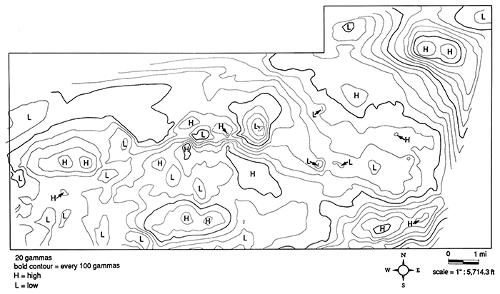
Magnetic data reduction consisted of removing the normal diurnal magnetic drifts and eliminating poor data from the data set. The magnetic data were then machine contoured (fig. 5) and a fishnet projection (fig. 6) was generated from the data.

The gravity data were reduced to simple Bouguer values (Dobrin, 1976). Corrections and adjustments were made for elevation, latitude, and tidal drift. Instrument drift was removed by using the base station and duplicated intersection readings. The data for the southeast Lawrence project were machine contoured (fig. 7). In the other two gravity projects, the data were hand contoured (figs. 3 and 4).

Gravity of the Gardner area

The Gardner gravity map (fig. 3) shows a variety of features. Most of the "high" features are 0.4-0.8 mgal elongated anomalies. The long axis generally trends north to northeast. Some of the features are narrow and ridgelike, while others are oval and domelike. Gravity lows either parallel the high trends or have a rather disorganized pattern. These trends (highs and lows) generally have spatial phase relationships (i.e. peak-to-peak or trough-to-trough), especially near the middle of the map, about 1 mi (1.6 km) in length.

Figure 3--Simple Bouguer gravity map northwest of Gardner, Kansas, located in west-central Johnson County.

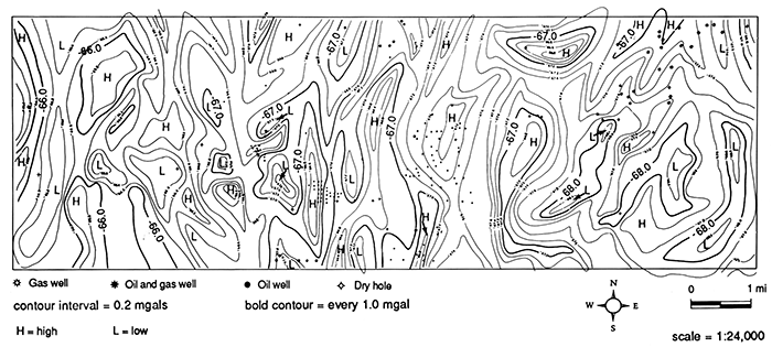
The general geologic structure through this county is a broad anticlinal feature trending north by northeast. Squirrel and Bartlesville oil sandstones often have this same trend with sand bodies 1/4-1 mi (.4-1.6 km) apart.

At least a few of these anomalous highs are associated with oil or gas fields. The Gardner dome is located 1 mi (1.6 km) east of center of the mapped area. The 0.4-mgal bean-shaped anomaly generally encompasses most of the cluster of oil wells around the dome (fig. 8). This 1,060-acre field, discovered in 1939, has produced over 521,800 bbls of oil from the Marmaton and Cherokee sandstones (Paul and Beene, 1983).

The northern part of the Gardner South oil field, south of the Gardner dome, is seen as a 0.4-mgal ridgelike gravity feature. This 120-acre field, discovered in 1938, produced 1,846 bbls of oil from three wells during 1982 (Paul and Beene, 1983). Recent drilling has extended this field north towards the Gardner dome. Production is from Cherokee sandstones.

Bartlesville oil is produced from 28 wells located near the center of a long north-south ridgelike gravity high located 1 mi (1.6 km) west of the center of the map. Oil production is from an 8-12 ft (2.4-3.6 m) zone about 870 ft (261 m) deep. Recent drilling 2 mi (3.2 km) north has extended this trend off the north edge of the map.

The most interesting feature in all three study areas is the large, 1.0-mgal gravity high located in the center of the northeast edge of this map (fig. 3). The kidney-shaped anomaly is 1 3/4 mi (2.8 km) long east to west and 3/4 mi (1.2 km) long north to south.

Drilling during 1982-83 in the northeast corner of this feature discovered three Cherokee gas wells with absolute open flow potential of 4.5 million ft³ (0.14 million m³) per day. Further drilling has produced an additional dozen gas wells in the eastern portion of this gravity feature. This field is an extension of the Olathe gas field.

Recent geochemical analysis (table 1) indicates the gases are derived from both thermogenic and biogenic mechanisms. These gases have similar characteristics to gas analyzed from Franklin and Lyon counties (Newell, personal communication, 1985).

Table 1--Geochemical gas analysis. Well--William #1, S2 NW sec. 6, T. 14 S., R. 23 E., Johnson County, Kansas; production zone--Pennsylvanian Bartlesville sandstone; production depth--790 ft (237 m).

Gravity of the Vinland area

Like the Gardner gravity data, the Vinland data (fig. 4) show a variety of gravity features. Most of the highs or lows have closures between 0.4 and 0.8 mgals with anticlinal or synclinal slopes.

Figure 4--Simple Bouguer gravity map located in southeastern Douglas County, Kansas.

The map shows a two-fold grain to the data. A moderately steep gradient trends from near the center of the bottom of the map toward the northwest corner. Several oblong closures along this trend are either parallel or perpendicular to this gradient.

Data northeast of the gradient reveal broad, low-amplitude ridgelike highs and troughs. The predominant orientation is northeast to southwest. This area resembles a plateau. The data southwest of the gradient have a long north to south high ridgelike trend with broad oval-shaped lows on both sides. This area has the same data texture as the Gardner area.

The Eudora South gas and oil field is a few miles north of the northeast corner of the map. The Baldwin oil field is a few miles south of the map area. Fewer than a dozen wells had been drilled within the Vinland area before this study was conducted.

Several gravity features were selected for wildcat tests. The first oil discovery was on the H. Thoren lease in NE sec. 6, T. 14 S., R. 21 E., roughly 5 mi (8 km) south of Eudora, Kansas. The lease straddles the broad gravity ridge in the northeast corner of the map. Oil production was found in a 14-ft (4.2-m)-thick Cherokee sandstone at a depth of about 800 ft (240 m). Initial production ranged between five and 10 bbls per day while long-term production is one to two bbls per day. Notably, the third well had a strong 35 BOPD flush lasting over a month's time.

During 1984 a large number of wells (estimated to be over 100) were drilled in this area between Baldwin and Eudora. Several new pools are now producing oil from the Cherokee sandstones.

Gravity and magnetics of the southeast Lawrence area

Like the other two maps, the southeast Lawrence gravity and magnetic maps (figs. 5-7) show a variety of features. Gravity highs and lows have slightly larger amplitudes than the other two areas, ranging between 0.4 to 1.4 mgal closures. The areas of these anomalies also are larger, varying from 200 to 3,000 acres.

Figure 5--Magnetic map located in east-central Douglas County. Lawrence, Kansas, is located in extreme northwest corner of map.

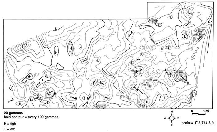
Figure 6--Fishnet projection of magnetic data in east-central Douglas County.

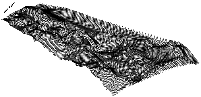
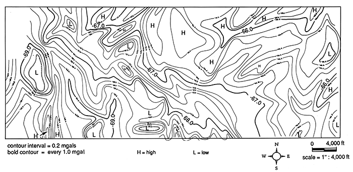
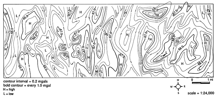
Figure 7--Simple Bouguer gravity map of east-central Douglas County, Kansas.

The gravity is split between two data textures. As on the Vinland map, a relatively steep gradient cuts the two textures. This gradient starts at the bottom of the map east of the center and continues in a curvilinear pattern northward to the map's edge.

Data in the eastern third of the mapped area, east of the gradient, reveal several large dome-shaped gravity highs, especially in the southern half. The town of Eudora is located near the center of the northern half of this area. The Eudora and Eudora South gas pools cover most of the eastern third of the map.

Data in the middle third section express a broad gravity low with only small-amplitude anomalies. Regional data grain is in a north-south direction.

The western third of the southeast Lawrence data set again expresses dome-shaped high anomalies in the southern part. The anomalies range between 300 and 500 acres in closure size. A large circular gravity high (1.0 mgal) is located over the town of Lawrence in the extreme northwest corner of the mapped area. The Lawrence gas pool is located east of the feature. In early 1984, most of the western two-thirds of the area had not been drilled. Even by late 1984, very few wells had tested any zone below the Cherokee section.

The magnetic data (figs. 5 and 6) show slightly different geophysical trends and features. The overall trend of the features and gradient is east to west. The anomalies are large (3-6 mi²; 7.8-15.6 km²) features with amplitude closures between 40 and 100 gammas. In the southeast corner, a 100-gamma anomaly, covering over 6 mi² (15.6 km²), corresponds to the highs on the gravity map over the Eudora South gas pool. The large magnetic high in the northeast is located over or near the Eudora gas pool. The other two large magnetic-high features, in the western half of the map, are located in undrilled areas.

The magnetic data were projected into a fishnet perspective diagram (fig. 6). This diagram projected the data as a surface from a viewpoint in the southeast corner of the mapped area and 30° above the surface. All the contoured anomalies previously discussed are seen as hills, valleys, and slopes. Because of the projection process, the amplitudes and horizontal dimensions are distorted across the fishnet.

Interpretation

Although the relationship between the magnetic and gravity fields and the oil and gas pools is unclear, it is probably one of the following:

1. The apparent association of gravity and magnetic highs with oil and gas pools may be coincidental. The occurrence of hydrocarbons in the Cherokee sandstone is thought to be largely stratigraphically controlled with little or no structural influence. If this is the case, there should be only a coincidental relationship between the gravity and magnetic fields and the oil pools (Gardner dome, Gardner South, gas wells north edge of fig. 3, and wildcat discovery in fig. 4).
2. The second possible relationship is of a structural nature. The gravity and magnetic features have dimensions of a few thousand to 10,000 ft (3,000 m). The lateral sizes of the gravity features associated with the oil and gas pools in the Gardner area (fig. 3) (Gardner dome, Gardner South and gas wells on north edge of map) are 4,000-8,000 ft (1,200-2,400 m). Generally this also constrains the depth of buried rock mass producing the gravity anomaly. Thus, these features are well within Precambrian granite rock, which was reached at a depth of 2,400 ft (720 m) in a well in sec. 12, T. 14 S., R. 22 E., 2 mi (3.2 km) north of Gardner, Kansas. These features are likely produced from the emplacement of denser rock into the granite crust. The age of the emplacement of these denser masses is important. If the emplacement is Precambrian (before sediment deposition), then weak vertical zones (faults or rock-contact surfaces) are likely to be found bounding the edges of these features. Therefore, vertical movement in the granitic and sedimentary rocks would likely occur along these weak vertical zones. This movement, if it occurred post-Pennsylvanian, would produce structurally high sand bodies over the gravity anomalies. It would also produce even larger amplitude structural traps in deeper pre-Pennsylvanian rocks. Detailed mapping of the Pennsylvanian formations indicates broad low-amplitude features. The anticlinal and synclinal features have closures of only 10-50 ft (3-15 m; Stander, 1983, unpublished data). Cherokee sandstone bodies are likely to contain hydrocarbons when they cross an anticlinal feature. If the age of the emplacement of the gravity anomalies is postdeposition, then the emplacement of the denser rock mass into the granite mass would likely cause a vertical movement in the sedimentary section above. This movement would produce structural traps above the gravity anomalies. The traps (anticlines) would have equal magnitude throughout the sedimentary section if the movement occurred only once after deposition (i.e. after Permian time). But if the movement occurred over geologic time, then the structural features would increase in magnitude with increasing depth. There are three reported cases in eastern Kansas of igneous rock masses intruding into the sedimentary sections during Cretaceous time. The Rose dome and Silver City lamproites are located in Woodson County (Jewett, 1954). Several kimberlite pipes are exposed in Riley County (Brookins, 1970). A more complicated structural interpretation is possible. It is likely that the gravity and magnetic anomalies were emplaced throughout geologic time. Some are Precambrian, while others are Cambrian to Cretaceous in age. If this is so, then not all of the gravity and magnetic features would have produced hydrocarbon traps in the overlying sediments.
3. A third possibility is that the gravity and magnetic anomalies are related in local high-heat producing features that generated the hydrocarbons. The source and generation of oil and gas in eastern Kansas is an unresolved question. If the hydrocarbons that are trapped in Cherokee sandstones are generated out of the surrounding Cherokee shales, then local heat sources are needed. The maximum depth of buried sediments in eastern Kansas would have occurred during the Cretaceous Period if the Cretaceous sediments extended themselves over eastern Kansas. Thus the maximum depth of the bottom of the Cherokee shales is estimated to be between 1,500 and 2,000 ft (450-600 m). The maximum temperature created by the normal geothermal gradient would not exceed 115° F (46° C). The normal temperature range throughout the Cherokee shales would vary between 80° F and 100° F (27-38° C) for depth of burial between 800 and 1,500 ft (240-450 m). Sediments with maximum temperature less than 122° F (50° C) are considered immature in the thermal alteration of kerogen into producible hydrocarbons (Hunt, 1979). The Cherokee shales would not be expected to generate many hydrocarbons through regional burial of sediment under normal geothermal gradients. In particular, gases are thermally generated at much higher temperatures than oil, ranging from 158° F to 392° F (70-200° C), with methane peaking at 302° F (150° C). Preliminary analysis of gas collected from the Cherokee gas well (William #1, sec. 6, T. 14 S., R. 23 E.) indicates the gas to have both a biogenic and a thermal source. Therefore, the source of the Cherokee oils and gases falls under the remaining possibilities: a) biogenic mechanisms, b) migration from much deeper Cherokee source beds, or c) generation from local high-heat areas. While biogenic generation and migration may be an important source of hydrocarbons in eastern Kansas, the thermal generation of hydrocarbons from local high-heat sources may be related to the gravity and magnetic anomalies. Gravity and magnetic highs (figs. 3-8) may outline or define historically high heat flow areas. These high heat flow areas could have generated enough heat locally to thermally produce hydrocarbons from the Cherokee shales. As in the structural interpretation, the timing of emplacement is important. If the gravity and magnetic features are Precambrian, then high heat flow could have occurred through vertical permeable zones such as faults or vertical rock contacts on the edges of the anomalies (Steeples, 1982). If the anomalies are post-Permian, the same age as the Cretaceous Riley County kimberlites, then the high heat flow would be derived from the emplacement of molten igneous rock into the Precambrian granitic crust. This type of emplacement would also produce doming in the overlying sediments. This emplacement of molten rock would create both the trapping mechanism and the heat source for hydrocarbon generation. The creation of the gravity and magnetic features may also have occurred throughout geologic time. The hydrocarbon generation may be a complex combination of high heat flow from vertical permeable zones surrounding Precambrian features to high heat flow from cooling of Cretaceous intrusive bodies.
4. The actual relationship between the oil and gas deposits and the gravity and magnetic features is probably a combination of the above three situations (coincidental, structural, and geothermal). Some of the geophysical features are likely to be coincidental without any bearing on hydrocarbon deposition. Another portion of the features is likely to be strictly of a structural nature of developing hydrocarbon traps. Additional features are likely related to high heat flow areas which generated the hydrocarbons trapped in nearby sandstones. Of course, the most attractive relationship from the standpoint of hydrocarbon exploration would be that the gravity and magnetic features are caused by the emplacement of Cretaceous molten igneous rock bodies. It is most attractive because it provides both the trapping mechanism and the heat source for the generation of hydrocarbons.

Figure 8--Simple Bouguer gravity map with oil and gas wells located in west-central Johnson County, Kansas.

Future research and exploration

The relationship between hydrocarbon pools and local gravity and magnetic fields is still unclear. Future research aimed at revealing this relationship would outline exploration strategies for finding additional hydrocarbons. Geochemical and maturation studies of both the hydrocarbons and shales over the geophysical anomalies would provide insight into their relationship. Deep CDP seismic surveys might uncover a structural relationship.

Future exploration for hydrocarbons in eastern Kansas would be influenced if the relationships could be understood. For example, if the gravity and magnetic features are Cretaceous intrusives, then geophysical surveys would outline not only the trapping structure, but also the heat source for the hydrocarbon generation. But, whatever the relationship, the gravity and magnetic features are attractive locations for deeper pre-Pennsylvanian drilling targets.

Conclusion

Three geophysical surveys were conducted in Johnson and Douglas counties, Kansas. The first two were gravity surveys and covered nearly 50 mi² (130 km²). The third project was a combination gravity and ground magnetic survey that covered nearly 110 mi² (286 km²).

The data were reduced and presented as contour maps. Data generated tended to parallel known structure trends. Gravity anomalies exhibited between 0.20 and 1.20 mgal closures. Magnetic features had closures of 60 to 80 gammas.

Known oil and gas pools (Gardner dome and Gardner South) were expressed in the gravity data as elongated oval-shaped 0.40-mgal closures. Several geophysical anomalies were selected as wildcat drilling sites. The first notable find was a discovery well of the Little Wakarusa Creek oil field south of Eudora, Kansas.

The exact relationship of the gravity and magnetic anomalies to the oil and gas field is not clear. But the geophysical anomalies are interpreted to be most likely a combination of two cases. First, the anomalies are Precambrian features with weak zones at the boundaries. Vertical movement has occurred in the weak zones causing structural traps to develop in overlying sediments. High heat flow would also be possible in these weak zones which would aid in the thermal alternation of the kerogen into hydrocarbons.

The other possibility is that the anomalies were created by intrusion of molten rock during Cretaceous time. The emplacement of molten rock in the granite basement would not only cause doming in overlying sediments, but would create a local heat source for hydrocarbon generation. Even without understanding the exact relationship between the geophysical features and present oil and gas pools, the survey provided useful data in selection of wildcat drilling sites in unexplored areas and depths.

References

Brookins, D. G., 1970, Kimberlites of Riley County: Kansas Geological Survey, Bulletin 200, 32 p. [available online]

Dobrin, M. B., 1976, Introduction to geophysical prospecting: McGraw-Hill Book Co., York, PA, p. 357-567.

Haworth, E., 1908, Special report on oil and gas: University Geological Survey of Kansas, p. 1-50.

Hunt, J. M., 1979, Petroleum geochemistry and geology: W. H. Freeman and Co., San Francisco, CA, p. 145.

Jewett, J. M., and Oros, M. O., 1954, Oil and gas in eastern Kansas: Kansas Geological Survey, Bulletin 104, p. 192-200, 239-244 (update written in 1979).

Paul, S. E., and Beene, D. L., 1983, 1982 oil and gas production in Kansas: Kansas Geological Survey, Energy Resource Series 23, p. 73.

Steeples, D. W., 1982, Structure of the Salina-Forest City interbasin boundary from seismic studies: UMR Journal, no. 3, p. 55-81.

Kansas Geological Survey
Comments to webadmin@kgs.ku.edu
Web version Sept. 12, 2013. Original publication date 1989.
URL=http://www.kgs.ku.edu/Publications/Bulletins/226/Stander/index.html