| Original published in D. W. Steeples, ed., 1989, Geophysics in Kansas: Kansas Geological Survey, Bulletin 226, pp. 267-295 | ||
Department of Geological Sciences, Southern Methodist University
The article is also available as an Acrobat PDF file.
Temperature, thermal-conductivity measurements, and heat-flow values are presented for four holes in Kansas originally drilled for cooperative water-resources investigations by the Kansas Geological Survey and the U.S. Geological Survey. These holes cut most of the sedimentary section and were cased and allowed to reach temperature equilibrium. Several types of geophysical logs were run for these holes. Temperature data from an additional five wells also are presented. Temperature gradients in the sedimentary section vary over a large range (over 4:1), and significantly different temperatures occur at the same depth in different portions of the state. Temperatures as high as 34°C (93°F) occur at a depth of 500 m (1,650 ft) in the south-central portion of the state but are 28°C (82°F) or lower at that depth in other parts of the state. In addition to cuttings measurements, thermal conductivities were estimated from geophysical well-log parameters; useful results suggest more use of the technique in the future. With these results, geophysical well logs can be used to predict temperatures as a function of depth in areas for which no temperatures are available if heat flow is assumed. The extreme variation in gradients observed in the holes occurs because of the large contrast in thermal-conductivity values. Shale thermal-conductivity values appear to have been overestimated in the past; Paleozoic shales in Kansas have thermal-conductivity values of approximately 1.18 ± 0.03 Wm-1K-1. Conversely, evaporite and dolomite units have thermal conductivities of over 4 Wm-1K-1. In spite of the large variations of gradient, the heat-flow values throughout the holes do not vary more than 10%, and any water-flow effects which might be present from the lateral motion on any of the aquifers are less than 10%. The best estimates for heat flow in the four holes come from carbonate units below the base of the Pennsylvanian and range in value from 48 mWm-2 to 62 mWm-2. Two of the holes were drilled to the basement, and correlation of the heat flow with basement radioactivity suggests that the heat-flow/heat-production line postulated for the midcontinent by Roy, Blackwell, and Birch (1968) applies to these data. Because of the low thermal conductivity of the shales, the radiogenic-pluton concept should apply to the midcontinent. Thus, if very radioactive plutons can be identified, much higher temperatures may occur in the sedimentary section than have been thought possible in the past. However, the past overestimation of the shale-conductivity values suggests that some previous high heat-flow values in the midcontinent probably are not correct, and the high gradients are due instead to normal heat flow and very low thermal-conductivity values. In spite of the presence of-low thermal-conductivity values in the midcontinent region, significant use could be made of geothermal energy in Kansas for space heating, thermal assistance, and heat-pump applications because the temperatures in the sedimentary section in much of Kansas are in excess of 40°C (104°F).
As of 1981, only two published heat-flow measurements were available for the state of Kansas. A value of 63 mWm-2 was measured near the central part of the state at Lyons, Kansas (Sass, Lachenbruch, and Munroe, 1971); a value of 59+ mWm-2 was estimated for a site near Syracuse by Birch (1947). Also, a heat-flow value of 59 mWm-2 was published by Roy, Decker, Blackwell, and Birch (1968) for a site in extreme northeastern Oklahoma near the Kansas border. On a regional basis, the eastern part of Kansas should be part of the Central Stable Region, an area of the North American continent characterized by a single linear relation between heat flow and heat production (Roy, Blackwell, and Birch, 1968). In this area, unless heat-flow values are disturbed, they are directly related to the heat production of the basement underlying the site where the heat-flow measurement was made.
Regional data suggest that heat flow may increase toward the west in the Great Plains province and that the high heat-flow characteristic of the southern Rocky Mountains may extend east of the mountains some distance (Blackwell, 1969; Combs and Simmons, 1973; Lachenbruch and Sass, 1977; Blackwell, 1978). Extensive thermal studies in the Great Plains in Nebraska, South Dakota, and North Dakota have been discussed by Gosnold (1985, 1989) and Gosnold and Eversoll (1982). In these three states, the surface heat flow is affected by regional fluid flow in the Cretaceous Dakota sand and the Mississippian carbonate aquifers. Swanberg and Morgan (1979) published a heat-flow map for the United States based on a correlation of heat flow and silica-water temperatures. In this map, they have a data gap for the state of Kansas, but extrapolation from data outside the state implies heat flow may be greater than 65 mWm-2 in the western part of the state and less than 65 mWm-2 in the eastern part. While no heat-flow measurements were made in western Kansas as part of this study in the area presumed to be characterized by heat flow above that of the Central Stable Region, the data presented here bear on the heat-flow values in the Great Plains, and this topic will be discussed in a subsequent section.
The plan of the U.S. Geological Survey and the Kansas Geological Survey to drill four deep hydrologic tests in Kansas prompted Dr. Don Steeples to propose a geothermal study for these wells. This study has been carried out by the authors of this report. These wells offer a unique opportunity to make detailed and accurate heat-flow measurements in Kansas. The wells were drilled through the Arbuckle Group to within a few feet of the basement. Two of the holes were drilled on into the basement, and core samples of basement rock were collected. The four holes are deep, have been cased through most of their depth, and have been left undisturbed to reach temperature equilibrium. Therefore, it is possible to get highly accurate, stable temperature measurements through the complete sedimentary section. This opportunity does not arise very often in the midcontinent, even though thousands of wells have been drilled there, because most of the holes were drilled for petroleum exploration and are not available for equilibrium-temperature studies. Water wells are usually shallower and do not cut nearly as thick a section or approach the basement. Possible circulation effects also may disturb the temperatures within the water wells.
In addition, an extensive suite of geophysical logs was obtained for each of the four holes (gamma ray, travel time, density, neutron porosity, electric, etc.), and cuttings were collected at frequent intervals. The holes which were drilled to the Arbuckle Group or deeper by the U.S. Geological Survey are NE NE SE sec. 13, T. 12 S., R. 17 E., SW SW SW sec. 32, T. 13 S., R. 2 W., SE SW SE sec. 18), T. 18 S., R. 23 E., and SW NE SW sec. 22, T. 31 S., R. 20 E. In addition, five other holes were logged as part of this study. For these holes, cutting samples and geophysical logs are not available, but the additional holes offer useful supplementary information on the temperature regime in Kansas.
The holes were logged to a maximum depth of 1,045 m (3,449 ft) with a truck-mounted logging system or to 565 m (1,865 ft) with portable hand-operated equipment. Most of the holes were logged with a digital-recording system attached to the output of the digital voltmeter attached to a thermistor probe and the output of a digital depth encoder. Temperatures were calculated from the measured resistance values and gradients were calculated using the two data sets. Temperatures were measured to the nearest 0.001 °C at depth intervals of 1 m (3.3 ft), allowing a very detailed look at gradients in the sedimentary section. Logging rates were quite slow, 4 m (13 ft) per minute, so that equilibrium temperatures were obtained. Blackwell and Spafford (1987) have described in detail the temperature logging and thermal-conductivity measuring equipment used in this study. Roy, Decker, et al. (1968) and many subsequent authors have illustrated the detail which can be obtained in sedimentary rocks using such continuously recording equipment.
Thermal-conductivity measurements were made on cuttings from three of the holes drilled by the Kansas Geological Survey and the U.S. Geological Survey. These results are given in appendix B. Only cuttings were available for the sedimentary section, so the measurements were made using the chip technique described by Sass, Lachenbruch, Munroe et al. (1971). Core samples were available from basement rock at two of the sites, and heat production and thermal conductivity were measured on the core samples. These data will be discussed below. Heat-production measurements were made using a 256-channel gamma-ray pulse-height analysis system (Gosnold, 1976). Core-sample thermal-conductivity measurements were made using conventional divided-bar techniques (Roy, Decker, et al., 1968). A major problem arose in the use of the chip technique to measure thermal conductivities for some of the units in the sedimentary section. Because of the strong anisotropy of the layered silicates making up the shales, obtaining the correct in situ thermal-conductivity values of the shales using cutting samples proved impossible. In preparing the cylinders with the mixture of water and cuttings, many shale fragments apparently will end up randomly orientated. However, when the shale is in the ground, the orientation is strongly preferred. The result is that the calculated in situ conductivity is far too high; this point is discussed in much more detail below.
In the tables showing interval thermal-conductivity values, these values have been corrected for temperature effects in the deeper parts of the holes (see Robertson, 1988). These effects approach 0.15 Wm-1K-1 for the bottom part of the hole in SW SW SW sec. 32, T. 13 S., R. 2 W.
Geothermal gradients were obtained in 10 relatively deep holes (375-1,045 m [1,238-3,449 ft]) throughout the eastern two-thirds of the state of Kansas. In all of these holes, temperature as a function of depth shows a very close relationship to lithologic variations. Because of this correlation and the thin-bedded nature of the Pennsylvanian section cut by most of the holes, it is very difficult to generalize the results. The hole locations and pertinent information are shown in table 1, and fig. 1 is a generalized index map of Kansas. The holes will be individually discussed proceeding in order from northwest to southeast. Bar graphs of gradient are shown for each hole. For the most detailed digitally recorded logs, temperatures are plotted at 2-m (7-ft) intervals.
Table 1--Location data for holes logged.
| Section, township, range |
North latitude |
West longitude |
Hole name |
Date logged |
Collar elevation (m) |
Depth logged (m) |
|---|---|---|---|---|---|---|
| NW SE SW sec. 27, 9S-20W | 39°14.7' | 99°32.6' | Rooks Co. | 11/15/1980 | 689 | 1,045 |
| NW NW SE sec. 13, 12S-17E | 39°00.8' | 95°28.7' | Big Springs | 11/25/1981 | 365 | 880 |
| SW SW SW sec. 32, 13S-2W | 38°52.3' | 97°34.5' | Smokyhill | 11/29/1981 | 369 | 1,044 |
| SE SW SE sec. 18, 18S-23E | 38°28.6' | 94°54.3' | Watson-1 | 6/9/1981 | 256 | 580 |
| sec. 23, 19S-8W* | 38°23.0' | 98°10.0' | LK-1 | 11/17/1970 | 525 | 229 |
| sec. 26, 19S-8W* | 38°22.0' | 98°10.0' | LK-2 | 11/17/1970 | 512 | 328 |
| SE NE SE sec. 34, 25S-4E | 37°49.8' | 99°58.3' | Butler Co. | 11/19/1980 | 405 | 737 |
| NE SW SW sec. 36, 25S-8E | 37°50.0' | 96°28.6' | Sallyard 9 | 11/19/1980 | 402 | 384 |
| NE SE SE sec. 24, 25S-13E | 37°51.6' | 95°55.4' | T.E. Bird | 11/18/1980 | 308 | 441 |
| SE SE SE sec. 2, 30S-24E | 37°27.4' | 94°44.5' | Frontenac | 1/10/1980 | 289 | 340 |
| SW NE SW sec. 22, 31S-20E | 37°19.8' | 95°12.4' | USGS-Bst | 6/4/1980 | 285 | 550 |
| *Data from Sass, Lachenbruch, and Munroe, 1971. | ||||||
Figure 1--Index map of sites of published heat-flow values (solid circles) and sites of holes discussed in this report (squares).
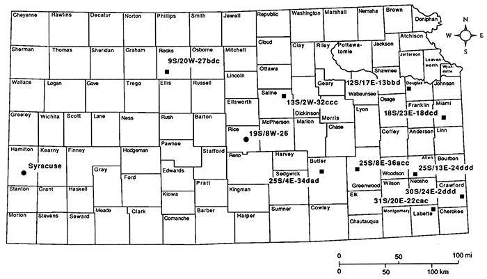
Fig. 2 shows a detailed temperature-depth curve and bar graph of gradient for the hole in NW SE SW sec. 27, T. 9 S., R. 20 W., in Rooks County. This hole was logged to the end of our cable at 1,045 m (3,449 ft). The upper part of the hole cuts Cretaceous rocks. The units which are most clearly identifiable on the temperature-depth and gradient plots in fig. 2 are the shales. The water level was just above 100 m (330 ft), and the first reliable gradients are below 105 m (347 ft). A 60-m (198-ft)-thick section between 105 m and 165 m (347-545 ft) has a mean gradient of 50.5 ± 0.3°C/km. Below that section the gradient drops to approximately 37.5 ± 0.5°C/ km to a depth of 221 m (729 ft), at which point the gradient drops to values generally less than 30°C/km, which continue to the bottom of the hole. The only exception is a zone of higher gradient between 300 and 340 m (990-1,122 ft) and a few local intervals of higher gradient between 900 and 1,000 m (2,970-3,300 ft), The Cretaceous-Permian unconformity is at a depth of approximately 950 m (1,485 ft) in this hole.
Figure 2--Temperature-depth and gradient-depth curves for the hole in NW SE SW sec. 27, T. 9 S., R. 20 W.; 1-m (3.3-ft) gradient intervals are plotted.
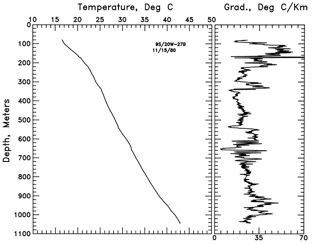
The mean gradient in the Cretaceous section (105-450 m [347-1,485 ft]) is 27.3 ± 1.8°C/km. In the Permian section (450-900 m [1,485-2,970 ft]), the mean gradient is 24.2 ± 0.3C/km, and in the Pennsylvanian section (900-1,045 m [2,970-3,449 ft]), the mean gradient is 33.6 ± 0.3°C/km. In the Pennsylvanian section, the gradients are variable ranging from 45°C/km in the predominantly shale units to 25°C/km in the more limestone-rich units. Temperatures are somewhat lower in this hole than in most of the other holes logged either because of a higher thermal conductivity for the Permian section, which includes more sandstone and evaporite deposits than the Pennsylvanian, or because of a lower heat flow at this site than at the remainder of the sites. The thermal-conductivity hypothesis is favored.
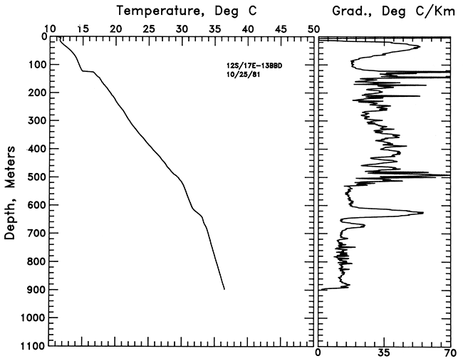
The hole in NW NW SE sec. 13, T. 12 S., R. 17 E., was drilled into Precambrian basement at a depth of 910 m (3,003 ft). The temperature-depth data and a bar graph of gradient for this hole are shown in fig. 3. The gradient in the Pennsylvanian section between 120 m and 521 m (396-1,719 ft) ranges from 25°C/km to just over 40°C/km and averages 32.1 ± 1.0°C/km. In the Mississippian carbonate section below 520 m (to 565 m [1,716-1,865 ft]), the mean gradient is 16.6 ± 0.1 °C/km. The gradient is 48.4 °C/km in the Chattanooga Shale and decreases abruptly to 12.6 ± 0.1 °C/km in the Arbuckle formation (predominantly dolomite).
Figure 3--Temperature-depth and gradient-depth curves for the hole in NW NW SE sec. 12, T. 12 S., R. 17 E.; 1-m (3.3-ft) gradient intervals smoothed by 3-point average are plotted.
Temperature-depth curves and bar graphs of gradient for the hole in SW SW SW sec. 32, T. 13 S., R. 12 W., are shown in fig. 4. This hole was drilled for the U.S. Geological Survey to a depth of 1,117 m (3,686 ft) and was logged to a depth of 1,044 m (3,445 ft). When this hole was logged, an injection test had recently been completed, and in the bottom part of the hole the temperatures were unstable, apparently because of this test. Some of the injected fluid entered the formation below 1,020 m (3,346 ft), resulting in the very high gradients in that section of the hole. The mean gradient between 100 and 280 m (330-924 ft) in the Permian section is 28.5 ± 0.6°C/km. The mean gradient in the Pennsylvanian section (280-792 m [924-2,614 ft]) is 31.9 ± 0.6°C/km.
Figure 4--Temperature-depth and gradient-depth curves for the hole in SW SW SW sec. 32, T. 13 S., R. 2 W.; 1-m (3.3-ft) gradient intervals smoothed by a 3-point running average are plotted.
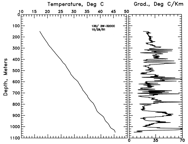
Below 792 m (2,614 ft) in the pre-Pennsylvanian section, the lithologic units are thicker, and a good correlation exists between lithology and gradient (fig. 4). The section of high gradient between 558 and 598 m (1,841-1,973 ft) corresponds to the Lawrence Shale. The gradient in this section is 48.6 ± 0.1 °C/km. The mean gradient between 736 and 796 m (2,429-2,627 ft) in the Cherokee Shale is 36.9 ± 0.2°C/km, while the mean gradient in the Chattanooga Shale between 862 and 912 m (2,845-3,010 ft) is 52.1 ± 0.1 °C/km. The mean gradient in the limestone units ranges from 15 to 25°C/ km. This hole was logged just into the Arbuckle Group (top at 1,026 m [3,386 ft]). The detailed geology and heat flow for this hole will be discussed in the following section.
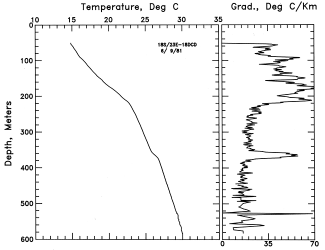
The hole in SE SW SE sec. 18, T. 18 S., R. 23 E.,was also one of the holes drilled for the U.S. Geological Survey. This hole was drilled into basement below 625 m (2,050 ft). The temperature-depth curve and a bar graph of gradient are shown in fig. 5. This hole shows generally high gradients ranging between 37 and 57°C/km and averaging 51.08 ± 1.2°C/km between 100 m and 220 m (330-726 ft), the Mississippian-Pennsylvanian contact. The gradient drops abruptly to average 22.7 ± 0.7°C/km in the remainder of the hole, with the exception of a 15-m (50-ft) section in the Chattanooga Shale. The average gradient in the Chattanooga Shale (360-375 m [1,188-1,238 ft]) is 51.5 ± 0.1 °C/km. Irregular gradients below 500 m (1,640 ft) reflect an injection disturbance. The mean gradient for the bottom of the hole below the Chattanooga Shale is 15.8 ± 0.1 °C/km. This section is predominantly dolomite as discussed in the section on heat flow. The hole was drilled into basement and bottomed at 666 m (2,200 ft). Basement thermal-conductivity and heat-production data are discussed below.
Figure 5--Temperature-depth and gradient-depth curves for the hole in SE SW SE sec. 18, T. 18 S., R. 23 E.; 1-m (3.3-ft) gradient intervals smoothed by a 3-point running average are plotted.
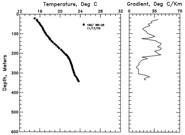
The hole in sec. 26, T. 19 S., R. 8 W., was logged, and the data presented by Sass et al. (1971). The temperature-depth and gradient data are shown in fig. 6; this hole was drilled in Permian-age rocks with the section of the hole between 220 and 305 m (725-1,000 ft) in salt deposits. Because of the high thermal conductivity of the salt, a low gradient of only 14 °C/km is observed within this interval.
Figure 6--Temperature-depth and gradient-depth curves for the hole in sec. 26, T. 19 S., R. 8 W. (Sass, Lachenbruch, and Munroe, 1971).
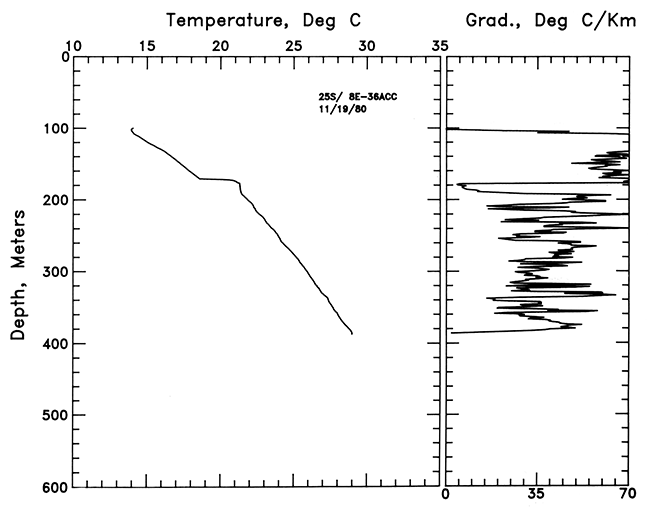
Three holes were logged along a more or less east-west section in the south-central part of the state located in SE NE SE sec. 34, T. 25 S., R. 4 E., NE SW SW sec. 36, T. 25 S., R. 8 E., and NE SE SE sec. 23, T. 25 S., R. 13 E. These holes are predominantly in Pennsylvanian-age rocks and have the highest temperatures in the 400-500-m (1,320-1,650 ft) depth range observed in any of the holes logged. In large part, the high temperatures are due to the greater abundance of low thermal-conductivity shale in the geologic section encountered in these holes. The temperature-depth curves and bar graphs of gradient for the first two holes are shown in figs. 7 and 8. The mean gradient for the hole in SE NE SE sec. 34, T. 25 S., R. 4 E., between 200 and 737 m (660-2,432 ft) is 35.6 ± 0.6°C/km. The gradients for SE NE SE sec. 34, T. 25 S., R.4 E., are quite variable; this hole was an abandoned oil well, and some of the irregularity may be related to past production effects. The character of the gradient variations changes abruptly at 310 m (1,023 ft). At this point a ball of mud or some other material apparently attached itself to the probe, severely lengthening the time constant of the probe and resulting in the marked change in behavior. The fluid level in the hole in NE SW SW sec. 36, T. 25 S., R. 8 E., was at 195 m (644 ft), and logging did not begin until below that depth. The mean gradient for that hole is 38.0 ± 0.4°C/km between 200 and 390 m (660-1,287 ft).
Figure 7--Temperature-depth and gradient-depth curves for the hole in SE NE SE sec. 34, T. 25 S., R. 4 E.; 2-m (7-ft) gradient intervals are plotted.
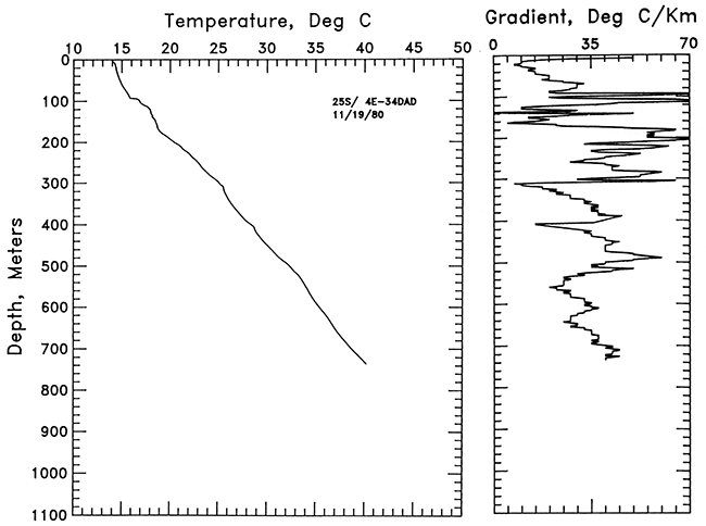
Figure 8--Temperature-depth and gradient-depth curves for the hole in NE SW SW sec. 36, T. 25 S., R. 8 E.; 1-m (3.3-ft) gradient intervals are plotted.
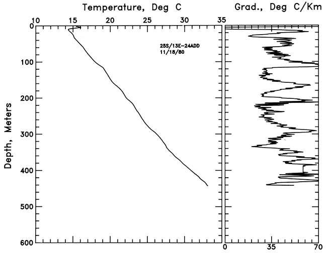
A temperature-depth curve and a gradient bar graph for the hole in NE SE SE sec. 24, T. 25 S., R. 13 E., are shown in fig. 9. In this hole there is a variation of 10-20-m (33-66-ft) interval gradients from about 25 to 55°C/km. From a comparison with the gamma-ray log, clearly these high gradients are closely correlated with sections of the hole which have higher gamma-ray activity, i.e. the shale sections. The sections of lower gamma-ray activity are predominantly limestone, although some sandstone may be represented by lower gamma-ray activity as well. The contacts between the shales and limestones appear quite sharp on the gamma-ray log above 150 m (495 ft) and not so sharp on the temperature log below 150 m (495 ft). This difference may be due to mud collecting on the probe and increasing the time constant, because this long-time constant-type behavior is not observed in the other holes logged (except the hole in SE NE SE sec. 34, T. 25 S., R. 4 E., see above) or in the upper part of this hole. The mean gradient for the hole between 40-441 m (132-1,455 ft) is 42.2 ± 0.9°C/km.
Figure 9--Temperature-depth and gradient-depth curves for the hole in NE SE SE sec. 24, T. 25 S., R. 13 E.; 1-m (3.3-ft) gradient intervals are plotted.
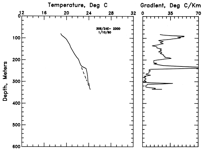
The only water well logged was the hole in SE SE SE sec. 2, T. 30 S., R. 24 E. This hole was logged to a depth of 340 m (1,122 ft). The temperature and gradient data are shown in fig. 10. Because the hole is an abandoned water well, the gradients may be disturbed by water circulation. From the shape of the temperature-depth curve, borehole upflow appears to occur between the bottom and about 220 m (726 ft), Not much is known of the section in this hole, but it is likely predominantly carbonate. The temperatures are quite low because it is one of the holes furthest to the east where the Pennsylvanian section is thinnest. The mean gradient between 105 and 340 m (347-1,122 ft) is 19.7 ± 1.6°C/km.
Figure 10--Temperature-depth and gradient-depth curves for the hole in SE SE SE sec. 2, T. 30 S., R. 24 E.; 2.5-m (8-ft) gradient intervals are plotted.
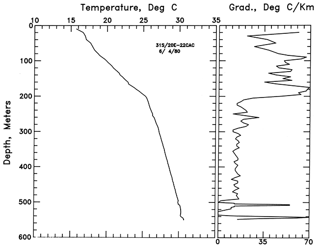
Extensive data are available for the hole in SW NE SW sec. 22, T. 31 S., R. 20 E., one of the holes drilled by the U.S. Geological Survey. This hole was logged to the drilled depth of 550 m (1,804 ft). The results are shown in fig. 11. The gradients between 95 m and 205 m (314-677 ft) are quite high, averaging 53.4 ± 1.5°C/km. Below 205 m (677 ft), the gradients average less than 20°C/km. The 205-m (677-ft) depth is the contact of the Pennsylvanian section with the predominantly limestone-dolomite section of Mississippian and older age. At the bottom of the hole are two negative-temperature excursions which are related either to drilling or injection. Because of the thinness of the high thermal-conductivity section, temperatures at depth are relatively low in this hole.
Figure 11--Temperature-depth and gradient-depth curves for the hole in SW NE SW sec. 22, T. 31 S., R. 20 E.; 5-m (17-ft) gradient intervals are plotted.
Using the data obtained directly from the logs, a table of temperatures at various depths was prepared (table 2). Temperatures are shown at depths of 400, 500, 750, and 1,000 m (1,320, 1,650, 2,475, and 3,300 ft) where available. Extrapolations have not been made except for very short depth intervals. Where extrapolations have been made, the numbers are given in parentheses. Most of the holes were logged to a depth of 400 m (1,320 ft), but only about two-thirds of them are logged to a depth of 500 m (1,650 ft). A contour map of temperature at 500 m (1,650 ft) is shown in fig. 12. At this depth, temperatures are highest in the southern third of the state except along the Missouri boundary. Temperature differences approach 6°C (43°F) at a depth of 500 m (1,650 ft). The mean surface temperature for almost all of the stations is between 13 and 15°C (55-59°F), and thus the mean gradients to 500 m (1,650 ft) range from approximately 40°C/km in the areas of highest temperature to only 28°C/km in the north-central portion of the state. However, these gradients cannot necessarily be projected to greater depths. Clearly vertical-gradient variations are due to lithology, and so very large variations in gradient will occur with depth. Furthermore, variations of heat flow may be related to other factors such as basement radioactivity. In order to evaluate some of these other variations, heat-flow values were calculated for several of the holes. These heat-flow values are discussed in the following section.
Figure 12--Isotherms at 500 m (1,650 ft); temperatures are in °C.
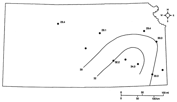
Table 2--Temperatures (°C) measured at selected depths. Extrapolated temperatures are in parentheses.
| Location | Depth (meters) | ||||
|---|---|---|---|---|---|
| 0 | 400 | 500 | 750 | 1000 | |
| NW SE SW sec. 27, 9S-20W | (14.0) | 26.2 | 28.4 | 34.2 | 41.8 |
| NW NW SE sec. 13, 12S-17E | 13.9 | 25.7 | 29.4 | ||
| SW SW SW sec. 32, 13S-2W | 14.0 | 25.8 | 29.1 | 37.1 | 45.2 |
| SE SW SE sec. 18, 18S-23E | (13.0) | 27.3 | (30.0) | ||
| sec. 26, 19S-SW | 15.0 | (25.5) | |||
| SE NE SE sec. 34, 25S-4E | (14.0) | 28.4 | 32.2 | 40.7 | |
| NE SW SW sec. 36, 25S-8E | (13.0) | 29.5 | |||
| NE SE SE sec. 24, 25S-13E | 14.0 | 30.8 | (34.0) | ||
| SE SE SE sec. 2, 30S-24E | (15.0) | 25.0 | |||
| SW NE SW sec. 2, 31S-20E | 15.0 | 28.6 | 30.0 | ||
Heat-flow values have been calculated for the four holes drilled by the U.S. Geological Survey. Thermal-conductivity measurements were made on cutting samples collected from all of the holes. The detailed results of the measurements are contained in the appendix. Suites of geophysical logs were run in all four of the holes, so log data were available to calculate the average in situ porosity for correction of bulk thermal conductivity to in situ thermal conductivity. Gradient segments chosen for averaging were selected from comparison of temperature-depth logs discussed in the previous section to geophysical logs and the geological analyses of cuttings from the wells.
In most cases, very good correlation exists between gradient and lithology, although in the Pennsylvanian section such a rapid vertical lithological variation takes place that in most cases the temperature data are not detailed enough to be identified with the individual units. This rapid vertical variation leads to difficulty in calculating heat flow because it is nearly impossible to isolate intervals composed only of one lithology over which heat-flow values can be reliably calculated. Where temperatures were measured in the Mississippian and older carbonate section, the thicker monolithologic units were suitable for heat-flow calculations, and the most reliable values come from these sections of the drill holes. The data for interval gradient, harmonic average thermal conductivity, and heat flow for each of the four holes are shown in tables 3-6. Generalized lithology for each interval is also listed. In general, the mean gradients in the carbonate sections of all the holes are nearly identical, averaging 17-21 °C/km in sections which are predominantly limestone and 13-17°C/km in sections which include dolomite. Gradients in the predominantly shale sections range from 35 to 53°C/km.
The results of interval geothermal gradient and heat-flow calculations for the hole in NW NW SE sec. 13, T. 12 S., R. 17 E., are shown in table 3. The values in the two thick carbonate sections above and below the Chattanooga Shale are similar (the average is 52 ± 3 mWm-2) and, as is the case in all the holes, much lower than the heat-flow values in the sections with a significant shale component. The reason for this difference is discussed further in the following paragraphs.
Table 3--Interval thermal conductivity, geothermal gradient, and heat flow for the hole in NW NW NW sec. 13, T. 12 S., R. 17 E. The thermal conductivity in column 2 is the value inferred from the best average heat flow divided by the gradient for that interval. Standard error listed with values.
| Depth interval, meters |
Φ | N | Thermal conductivity Wm-1K-1 |
Gradient mWm-1 |
Heat flow mWm-2 |
Generalized lithology |
|
|---|---|---|---|---|---|---|---|
| (1) | (2) | ||||||
| 120-145 | 0.10 | 1 | 2.36 | 1.17 | 41.0 ± 0.1 | 97 | Lawrence Shale |
| 145-165 | 0.10 | 1 | 2.91 | 1.85 | 26.0 ± 0.1 | 76 | predominantly limestone |
| 165-180 | 0.10 | 2 | 2.16 | 1.30 | 37.0 ± 0.1 | 80 | predominantly shale |
| 180-260 | 0.10 | 5 | 2.23 ± 0.12 | 1.64 | 29.2 ± 0.5 | 65 | predominantly limestone |
| 260-315 | 0.10 | 8 | 2.56 ± 0.10 | 1.88 | 25.5 ± 0.3 | 65 | predominantly limestone |
| 315-520 | 0.10 | 15 | 2.51 ± 0.15 | 1.34 | 35.8 ± 0.4 | 89.7 | Cherokee Shale |
| 520-600 | 0.06 | 11 | 2.90 ± 0.15 | 16.6 ± 0.1 | 48 | limestone and dolomite | |
| 610-640 | 0.06 | 3 | 2.40 ± 0.12 | 1.07 | 48.4 ± 0.5 | 116 | Chattanooga Shale |
| 695-880 | 0.08 | 16 | 4.40 ± 0.22 | 12.6 ± 0.1 | 55 | dolomite | |
| best heat-flow value | 52 ± 3 | ||||||
Table 4--Interval thermal conductivity, geothermal gradient, and heat flow for the hole in SW SW SW sec. 32, T. 13 S., R. 2 W. The values included in the heat-flow averages are indicated by the asterisks. The thermal conductivity in column 2 is the value inferred from the best average heat flow divided by the gradient for that interval. Standard error listed with values.
| Depth interval, meters |
Φ | N | Thermal conductivity Wm-1K-1 |
Gradient mWm-1 |
Heat flow mWm-2 |
Generalized lithology |
|
|---|---|---|---|---|---|---|---|
| (1) | (2) | ||||||
| 110-150 | 0.16 | 2 | 1.93 | 25.5 ± 0.3 | 49 | shale and limestone | |
| 150-275 | 0.12 | 4 | 2.20 ± 0.15 | 29.0 ± 0.2 | 64 | limestone and shale | |
| 150-455 | 34.4 ± 1.0 | shale and limestone | |||||
| 455-555 | 27.4 ± 0.3 | shale and limestone | |||||
| 558-598 | 0.09 | 2 | 2.44 | 1.17 | 48.6 ± 0.1 | 119 | Lawrence Shale |
| 598-634 | 0.09 | 1 | 2.25 | 26.9 ± 0.1 | 61 | limestone | |
| 634-644 | 0.06 | 1 | 2.60 | 31.3 ± 0.1 | 81 | conglomerate and shale | |
| 644-694 | 0.06 | 3 | 2.45 | 27.5 ± 0.1 | 67 | limestone and shale | |
| 694-710 | 34.6 ± 0.1 | shale and limestone | |||||
| 710-736 | 0.09 | 1 | 2.47 | 25.3 ± 0.1 | 62 | sandstone | |
| 736-796 | 0.09 | 2 | 2.31 | 1.54 | 37.0 ± 0.2 | 86 | Cherokee Shale |
| 796-862 | 0.10 | 20 | 2.97 ± 0.20 | 20.4 ± 0.3 | 61* | Mississippian limestone | |
| 862-912 | 0.06 | 2 | 2.30 | 1.09 | 52.2 ± 0.1 | 120 | Chattanooga Shale |
| 912-942 | 0.09 | 9 | 3.15 ± 0.25 | 17.3 ± 0.1 | 54* | Hunton Group | |
| 944-970 | 0.05 | 2 | 2.70 | 1.25 | 45.5 ± 0.1 | 123 | Sylvan Shale |
| 970-1044 | 0.06 | 21 | 2.92 ± 0.30 | 21.0 | 61* | Viola and Arbuckle groups | |
| best heat-flow value | 59 ± 3 | ||||||
The data for the hole in SE SW SE sec. 18, T. 18 S., R. 23 E., are shown in table 5. The heat flow calculated for the carbonate section is 60 mWm-2. The gradients in the Cherokee Shale and Chattanooga Shale are 52°C/km and the directly calculated heat-flow values are over 110 mWm-2. The heat flow on either side of the Chattanooga Shale is identical. If the true thermal conductivity for these two units is 1.15 ± 0.5 Wm-1K-1, then the heat flow in the shale units would be the same as in the carbonate units.
Table 5--Interval thermal conductivity, geothermal gradient, and heat flow for the hole in SE SW SE sec. 18, T. 18 S., R. 23 E. The values included in the heat-flow averages are indicated by the asterisks. The thermal conductivity in column 2 is the value inferred from the best average heat flow divided by the gradient for that interval. Standard error listed with values.
| Depth interval, meters |
Φ | N | Thermal conductivity Wm-1K-1 |
Gradient mWm-1 |
Heat flow mWm-2 |
Generalized lithology |
|
|---|---|---|---|---|---|---|---|
| (1) | (2) | ||||||
| 100-115 | 36.9 ± 0.1 | shale and limestone | |||||
| 115-220 | 0.12 | 7 | 2.25 ± 0.15 | 1.15 | 52.4 ± 1.1 | 115 | Cherokee Shale |
| 220-360 | 0.10 | 10 | 2.84 ± 0.20 | 23.2 ± 0.4 | 59* | Mississippian limestone and dolomite | |
| 360-375 | 0.06 | 2 | 2.24 | 1.14 | 52.5 ± 0.1 | 118 | Chattanooga Shale |
| 380-580 | 0.10 | 7 | 3.90 ± 0.20 | 15.8 ± 0.1 | 62* | dolomite | |
| best heat-flow value | 60 ± 3 | ||||||
The data for the hole in SW NE SW sec. 22, T. 31 S., R. 20 E., are shown in table 6. Thermal-conductivity measurements are made on samples from the Arbuckle Group. The rock is adense dolomite with a high thermal conductivity so that even though a large interval (290-550 m [957-1,815 ft]) has a low gradient, the heat flow is the highest (by only 3%) of all the values obtained. The gradients are slightly higher in the limestone section of the hole above the dolomite, and much higher (by a factor of over 4) in the Cherokee Shale. The inferred thermal conductivity of the shale is shown in parentheses. The gradients in the Arbuckle section are exactly the same in this hole and in two holes discussed by Roy, Decker, et al. (1968; see Decker and Roy, 1974) near Picher, Oklahoma, about 50 km (30 mi) to the southeast. The heat-flow values also are similar so that apparently the Arbuckle thermal conductivity is very similar in both holes. The heat flow for the holes discussed by Roy, Decker, et al. (1968) was based on thermal-conductivity measurements of core samples from Precambrian basement rocks.
Table 6--Interval thermal conductivity, geothermal gradient, and heat flow for hole in SW NE SW sec. 22, T. 31 S., R. 20 E. Thermal-conductivity value estimated as discussed in text.
| Depth interval, meters |
Φ | N | Thermal conductivity Wm-1K-1 |
Gradient mWm-1 |
Heat flow mWm-2 |
Generalized lithology |
|
|---|---|---|---|---|---|---|---|
| (1) | (2) | ||||||
| 70-205 | 0.12 | 12 | 2.47 ± 0.15 | 1.16 | 53.4 ± 1.5 | 132 | Cherokee Shale |
| 205-275 | 0.15 | 9 | 3.39 ± 0.40 | 20.5 ± 0.1 | 63 | Mississippian limestone and dolomite | |
| 290-550 | 0.08 | 17 | 4.46 ± 0.50 | 14.0 | 62 | Arbuckle dolomite | |
| best heat-flow value | 62 ± 6 | ||||||
The mean value for all the carbonate sections ranges from 48 to 62 mWm-2. Thus, on the basis of this analysis, only minor variation of heat flow would seem to occur among the four holes. However, if heat-flow values are calculated from thermal-conductivity measurements on cuttings from the pre-Pennsylvanian shale sections or from the Pennsylvanian units in each hole, then an extremely different picture of the heat flow is obtained. Typical cuttings determined thermal conductivities for the shale sections, using a porosity measured in situ of 10% ± 5% are 1.8-2.25 Wm-1K-1. These values taken together with typical gradients of 45-55°C/km imply heat-flow values in shale sequences of 100 mWm-2 or greater. These values are in clear contradiction to the heat-flow values obtained in the carbonate units.
Two possibilities exist for the differences in heat flow in the different lithologies. First a difference may exist in heat flow between the upper and lower parts of the drill holes. One of the reasons for drilling the wells was to investigate possible fluid flow in the Arbuckle aquifer; slow fluid motions could change the heat flow, resulting in lower or higher heat-flow values above the aquifer and also affecting heat-flow values below the aquifer. The second possibility is that the thermal conductivity of the shales is incorrectly estimated by the chip technique.
According to the first hypothesis, a change in heat flow should occur in association with the contact between the relatively impermeable shale section and the lower, more permeable, dominantly carbonate section. This hypothesis is untenable, however, because in three of the holes the high and low heat flow zones are interlayered, not sequential, and are exactly related to lithology, not permeability. Thus the problem seems to be with the measurement of shale thermal conductivity using the chip technique.
In conclusion, the range of thermal conductivity inferred for the shales encountered in the holes is between 1.1 and 1.3 Wm-1K-1. Thus, there is an approximate ratio of 2.5:1 between the thermal conductivity of the limestone and shale, and up to 4:1 between the thermal conductivity of dolomite and shale. Corresponding ratios of gradients in the various units are observed.
An examination of the chip technique of thermal-conductivity measurements indicates that not surprisingly, the shale conductivity will be in error. Since small fragments of shale are packed into a hollow cylinder, some of them may be on end and all of them are finite in length; therefore, conduction along the grains in the high-conductivity directions may be important. It is also difficult to measure thermal conductivity on core samples of shales, and perusal of the literature indicates adequate thermal-conductivity measurements for shale may not exist. It is difficult to measure shale thermal conductivity on the divided-bar using core samples because of the fissility of the shale. The anisotropy makes needle-probe measurements of dubious value. In heat-flow studies in the midcontinent, previous investigators have estimated the conductivity of the shale sections between 1.55 and 1.85 Wm-1K-1 (Garland and Lennox, 1962; Combs and Simmons, 1973; Scattolini, 1978). Judge and Beck (1973) encountered the problem in a study of heat flow in the Western Ontario basin where the rocks range in age from Precambrian to Mississippian. They found heat-flow values 60% too high in the Ordovician shale section (Collingwood Formation). If a value of 1.1 Wm-1K-1 is assumed as determined above for the lower Paleozoic shales in this study, the heat flow in the Collingwood Formation is the same as in the remainder of the units they studied (dominantly limestone and dolomite). Thus, the shale thermal-conductivity values in the literature are significantly in error. One implication is that the heat flow in the Great Plains may not be as high as has been estimated in the past. In particular, the zone of high heat flow extending out into the Great Plains, north of the Black Hills (Lachenbruch and Sass, 1977; Blackwell, 1978), may not exist. Furthermore, the correlation of silica values of ground water and heat flow for the midcontinent may be, instead, a correlation of silica values and mean geothermal gradient.
Even though high-quality temperature data exist, the conventional heat-flow values for the four holes must be based only on limited sections of the hole. Large sections of the hole cannot be used for heat-flow determinations by conventional heat-flow techniques. In the next section, use of well-log parameters combined with temperature data will be investigated to more completely evaluate the best heat-flow values for these four holes.
Difficulties in evaluating mean thermal conductivity in the shale sections and in sections with very rapidly varying thermal conductivity make it useful to have other techniques to evaluate these sections. Four of the holes had available extensive geophysical well-log suites, and use of these data to assist in calculation of the heat-flow values was investigated. It has been demonstrated in a number of studies that of various physical properties such as density, porosity, and velocity, velocity is most directly useful in estimating thermal conductivity (Goss and Combs, 1976; Williams, 1981), so emphasis was placed on use of the velocity and gamma-ray logs. The gamma-ray activity in these holes is relatively directly related to the amount of shale. Typical gamma-ray counts for the shale sections are about 100 ± 25 API units, whereas in the carbonate sections, gamma-ray values are 25 ± 5 API units. If the primary control on the thermal conductivity is the mixing of only two lithologies, then it should be possible to obtain a good correlation between gamma-ray activity and the gradient.
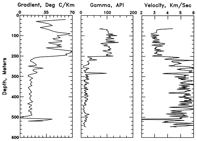
A series of bar graphs of temperature gradient, gamma-ray activity, and velocity for the four wells drilled for the U.S. Geological Survey are shown in figs. 13, 14, 15, and 17. For holes logged with digital equipment, gradient graphs are plotted using a running 2-m (7-ft) average. In addition, the gradient data from the hole in NE SE SE sec. 24, T. 25 S., R 13 E., are accompanied by a gamma-ray log from a nearby hole (fig. 16). The geophysical logs are based on a 0.5-m (1.7-ft) digitization of paper copies at a 5 inches = 100-ft (1:240) scale. The values plotted are 3-m (10-ft) running averages. Detailed evaluation of individual figures illustrates an almost point-by-point correlation between various regions of high gamma-ray activity, low velocity, and high geothermal gradient from the sections of the holes below 100-150 m (330-495 ft).
Figure 13--Comparison of geothermal gradient, gamma-ray activity, and P-wave velocity for the hole in NW NW SE sec. 13, T. 12 S., R. 17 E. The gamma-ray and P-wave data are based on 0.5-m (1.7-ft) digitized well logs smoothed by a 7-point average. Gradient plot from fig. 3.
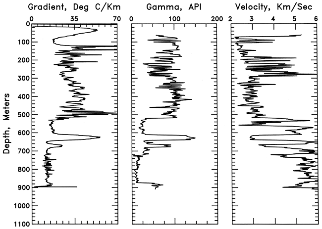
Figure 14--Comparison of geothermal gradient, gamma-ray activity, and P-wave velocity for the hole in SW SW SW sec. 32, T. 13 S., R. 2 W. The gamma-ray and P-wave data are based on 0.5-m (1.7-ft) digitized well logs smoothed by a 7-point average. Gradient plot from fig. 4.
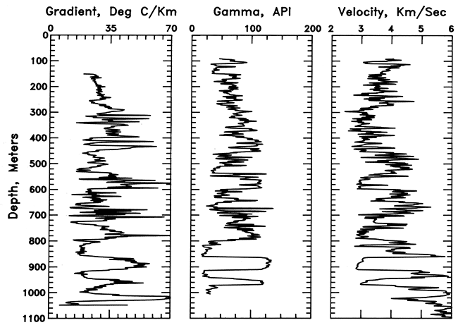
Figure 15--Comparison of geothermal gradient, gamma-ray activity, and P-wave velocity for the hole in SE SW SE sec. 18, T. 18 S., R. 23 E. The gamma-ray and P-wave data are based on 0.5-m (1.7-ft) digitized well logs smoothed by a 7-point average. Gradient plot from fig. 5.
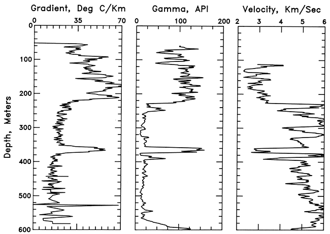
Figure 16--Comparison of geothermal gradient and gamma-ray activity for the hole in NE SE SE sec. 24, T. 25 S., R. 13 E. The gamma-ray data are based on 0.5-m (1.7-ft) digitized well logs smoothed by a 7-point average. Gradients are from fig. 9. The gamma-ray log is for a hole in SE NW NW sec. 24, T. 25 S., R. 13 E.
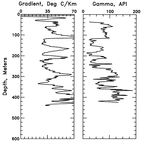
Figure 17--Comparison of geothermal gradient, gamma-ray activity, and P-wave velocity for the hole in SW NE SW sec. 22, T. 31 S., R. 20 E. The gamma-ray and P-wave data are based on 0.5-m (1.7-ft) digitized well logs smoothed by a 7-point average. Gradient plot is from fig. 11.
The bottom part (500-1,045 m [1,650-3,449 ft]) of the hole in SW SW SW sec. 32, T. 13 S., R. 2 W., shows the clear correlation between gradient, gamma-ray activity, and velocity in the Lawrence, Cherokee, Chattanooga, and Sylvan shales and the interlayered carbonate sections. In the hole in SE SW SE sec. 18, T. 18 S., R. 23 E., a very good correlation can be seen between the carbonate and shale units. In particular, the Chattanooga Shale stands out because of the extreme excursion in gradient, gamma-ray activity, and travel time in the midst of a predominantly carbonate section. The logs from the hole in NE SE SE sec. 24, T. 25 S., R. 13 E., also show a one-for-one correlation between areas of high gradient and high gamma-ray activity; however, because of the apparently impaired time constant of the probe, the shale-limestone contacts do not appear as sharp on the thermal log as on the gamma-ray log.
These visual relationships were quantified by utilizing crossplots prepared between velocity, travel time (inverse of velocity), gamma-ray activity, and gradient (figs. 18-21). Least-square straight-line fit to crossplots are depicted of the data averaged over 10-m (33-ft) intervals in the section of the hole for which both geothermal-gradient and geophysical-log data are available. In addition to the least-square straight line, the scatter of points for each hole is indicated by the corresponding envelope. Clearly, very systematic relationships exist between the four different properties, especially the gamma-ray activity and gradient.
Figure 18--Crossplot of 10-m (33-ft) averages of gamma-ray activity and geothermal gradients. Least-square straight-line fit to data and range of data are shown for each hole. Data from the hole in NW NW SE sec. 13, T. 12 S., R. 17 E. (100-560-m depth range), are shown as the light solid line, data from SW SW SW sec. 32, T. 13 S., R. 2 W., are shown as the heavy solid line, data from SE SW SE sec. 18, T. 18 S., R. 23 E. (100-400-m depth range), are shown as the dashed line, and data from SW NE SW sec. 22, T. 31 S., R. 20 E., are shown as the dotted lines.
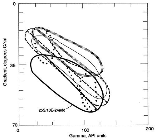
Figure 19--Crossplot of 10-m (33-ft) averages of compressional-velocity and geothermal gradient. The key is the same as in fig. 18.
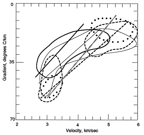
Figure 2O--Crossplot of 10-m (33-ft) averages transit time (msec/ft) and geothermal gradient. Least-square straight-line fit to data and range of data are shown on each hole. Data from NWNW SE sec. 13, T. 12 S., R. 17 E. (100-560-m depth range), are shown as the light solid line, data from SW SW SW sec. 32, T. 13 S., R. 2 W., are shown as the heavy solid line, data from SE SW SE sec. 18, T. 18 S., R. 23 E. (100-400-m depth range), are shown as the dashed line, and data from SW NE SW sec. 22, T. 31 S., R. 20 E., are shown as the dotted lines.
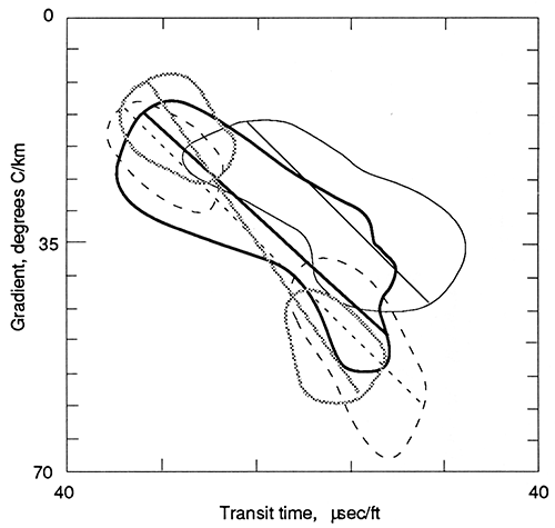
Figure 21--Crossplot of 10-m (33-ft) averages of gamma-ray activity and compressional velocity. The key is the same as in fig. 20.
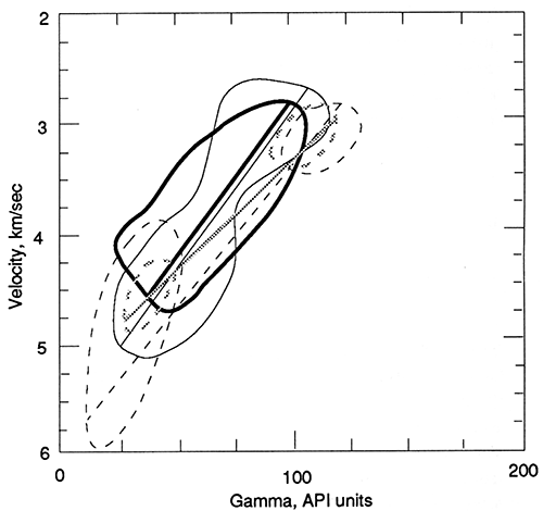
The relationship between gamma-ray activity and geothermal gradient is shown in fig. 18. All of the holes appear to have similar populations of gradient and gamma-ray data. The slopes of three of the holes are almost identical, and the lines are offset by approximately 5°C/km. The slopes for the holes in NE SE SE sec. 24, T. 25 S., R. 13 E., and SW NE SW sec. 22, T. 31 S., R. 20 E., are somewhat greater. However, the calibration of the gamma-ray data for the hole in NE SE SE sec. 24, T. 25 S., R. 13 E., is uncertain and a time-constant difficulty may exist with the temperature log. Based on the least-square-fit straight lines, a small variation in parameters can be found among the different drill holes. This variation could be due to systematic problems in calibration of the gamma-ray logs, lateral variations in gamma-ray-activity gradient, or thermal conductivity in the various units.
Some of these possibilities were evaluated by examining the relationship between velocity and geothermal gradient (see fig. 19). A very similar array of data is seen, i.e. similar slopes and an approximately 10°C/km offset in the lines. However, the total data envelope is not as clearly linear as is the case in fig. 18, especially for the holes in NW NW SE sec. 13, T. 12 S., R. 17 E. and SW SW SW sec. 32, T. 13 S., R. 2 W. The crossplots of gradient and transit time are shown in fig. 20. The envelopes of data points are more linear than in fig. 19. Again, the data overlap is almost complete for the holes in SW SW SW sec. 32, T. 13 S., R. 2 W., SE SE SE sec.18, T. 18 S., R. 23 E., and SW NE SW sec. 22, T. 31 S., R. 20 E., while the hole in NW NW SE sec. 13, T. 12 S., R. 17 E., has a best-fit line offset about 5°C/km below the other three lines.
Fig. 21 shows a correlation between gamma-ray activity and velocity. The data from the holes in NW NW SE sec. 13, T. 12 S., R. 17 E., and SW SW SW sec. 32, T. 13 S., R. 2 W., are identical, the one in SW NE SW sec. 22, T. 31 S., R. 20 E., is slightly steeper in slope and the one in SE SE SE sec. 18, T. 18 S., R. 23 E., is displaced by approximately 0.3 km/sec from the other lines. In this case, almost a complete overlap of all of the data sets occurs and apparently the same population of gamma-ray and velocity data are present in all of the holes.
The qualitative result of this investigation, using the indicators of velocity (transit time) and gamma-ray activity, provides the same order of results. The hole in NW NW SE sec. 13, T. 12 S., R. 17 E., has consistently the lowest gradient by 4-7°C/km. The hole in SW SW SW sec. 32, T. 13 S., R. 2 W., has the next lowest gradient by 2-5°C/km, and the hole in SE SE SE sec. 18, T. 18 S., R. 23 E., has the highest gradient. Gradients from the hole in SW NE SW sec. 22, T. 31 S., R. 20 E., overlap the data from the last two holes, being closer to the results for the one in SE SE SE sec. 18, T. 18 S., R. 23 E., at the high-gradient end and closer to the hole in SW SW SW sec. 32, T. 13 S., R. 2 W., on the gradient region of each curve. The heat-flow values from the pre-Pennsylvanian carbonate sections of each hole are shown in table 7a. The relative heat-flow values are similarly correlated as the normalized for log-response gradients as summarized in table 7b for the complete holes shown in figs. 18-20.
Table 7a--Adopted values of heat flow.
| Location | Best heat-flow values mWm-2 (µcal/cm2sec) |
Estimated error mWm-2 |
|---|---|---|
| NW NW SE sec. 13, 12S-17E | 52 (1.24) | ± 3 |
| SW SW SW sec. 32, 13S-2W | 59 (1.36) | ± 6 |
| SE SW SE sec. 18, 18S-23E | 60 (1.43) | ± 3 |
| SW NE SW sec. 22, 31S-20E | 62 (1.48) | ± 5 |
Table 7b--Heat flow derived from temperature and transit-time logs using the procedure described in the text.
| Location | Depth interval, meters |
Heat flow mWm-2 |
|---|---|---|
| NW NW SE sec. 13, 12S-17E | 120-550 | 40 |
| SW SW SW sec. 32, 13S-2W | 270-780 | 50 |
| 780-1000 | 54 | |
| 270-1000 | 50 | |
| SE SW SE sec. 18, 18S-23E | 110-3S0 | 61 |
| SW NES W sec. 22, 31S-20E | 70-290 | 66 |
Relative relationships of all of the holes (except that in SW NE SW sec. 22, T. 31 S., R. 20 E.) are evidence that the relative heat-flow values in table 7b are correct, even if the absolute heat-flow values are not. The similar relationship between the gradient and velocity/gamma ray above and below the Mississippian-Pennsylvanian contact is strong evidence against the possibility that the heat flow is much higher above than below the Mississippian-Pennsylvanian contact. Detailed analysis of the data shown in figs. 18-20 depends on the number of different lithologies involved. If only shale and limestone are present, then the analysis is relatively simple, and fortunately in this case these lithologies predominate. Minor components which may be locally important and cause difficulty in the interpretation are sandstone (higher thermal conductivity for a given velocity than the shale-limestone relationship), dolomite (higher thermal conductivity), and coal or lignite (lower thermal conductivity). Heat-flow values in table 7b were calculated using the relationship between thermal resistance (RT in cm sec°C/mcal and transit time in µsec/foot)
RT = -140+4.83t
and the relationship
T(x) = Q ∫0x RTdx.
Heat flow (Q) was calculated by a least-square, straight-line fit to T(x) versus the integral values. The results are shown in table 7b. Heat-flow values in table 7a agree within 20%, so that the heat-flow values using the data from the whole section in each hole are within 20% of the heat flow derived from the carbonate sections alone and are both higher and lower. A variation occurs in the response of the Pennsylvanian section in the holes in NW NW SE sec. 13, T. 12 S., R. 17 E., and SW SW SW sec. 32, T. 13 S., R. 2 W., as compared to holes in SE SE SE sec. 13, T. 8 S., R. 23 E.,and SW NE SW sec. 22, T. 31 S., R. 20 E., in that apparent thermal conductivities are higher for the first two holes than for the latter two. Either a slight change in heat flow at the Pennsylvanian-Mississippian contact (<5-10 mWm-2) occurs in the latter two holes or the lithology of the sections is different. A higher proportion of sandstone in the first two holes or coal in the second two (or a combination of both) is the most likely explanation of the apparent thermal-conductivity discrepancy.
Results of the analysis confirm a major conclusion from the previous section that shale thermal-conductivity values are overestimated by the chip technique of measurement and verify that heat-flow values are the same in different units if realistic values of thermal conductivity are assumed for the shale sections. The inferred thermal-conductivity values, average gradients, and thicknesses for the main shale units encountered are shown in table 8. With the exception of the Cherokee Shale in the holes in NW NW SE sec. 13, T. 12 S., R. 17 E., and SW SW SW sec. 32, T. 3 S., R. 2 W., all values are less than 1.3 Wm-1K-1 and the average value, excluding the Cherokee Shale in SW SW SW sec. 32, T. 13 S., R. 2 W., is 1.18 Wm-1K-1. The discrepancy of the Pennsylvanian sections was discussed in the previous paragraph, and the results in table 8 emphasize the apparent difference in the lithology of the Cherokee Shale in the two sets of holes.
Table 8--Inferred values of thermal conductivity (K), observed geothermal gradients (G), and thicknesses (t), The three quantities are shown for each shale unit in order, for each hole in which the shale occurs. The mean shale thermal conductivity (excluding the Cherokee Shale in SW SW SW sec. 32, T. 13 S., R. 2 W., is 1.18 ± 0.03 Wm-1K-1 (2.82 ± 0.07 mcal/cm sec°C).
| Location | Lawrence | Cherokee | Chattanooga | Sylvan | ||||||||
|---|---|---|---|---|---|---|---|---|---|---|---|---|
| K | G | t | K | G | t | K | G | t | K | G | t | |
| NW NW SE sec. 13, 12S-17E | 1.17 | 41 | 25 | 1.34 | 36 | 200 | 1.09 | 48 | 30 | |||
| SW SW SW sec. 32, 13S-2W | 1.17 | 49 | 40 | (1.54) | 37 | 60 | 1.09 | 52 | 50 | 1.25 | 46 | 26 |
| SE SW SE sec. 18, 18S-23E | 1.15 | 52 | 105 | 1.14 | 53 | 15 | ||||||
| SW SW SW sec. 22, 31S-20E | 1.10 | 53 | 135 | |||||||||
| K, Wm-1K-1 G, °C/km t, meters |
||||||||||||
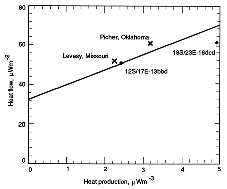
The heat-flow values obtained are shown in fig. 22 on a map which includes the simplified geology and the Precambrian basement rocks in Kansas. If nonconductive effects are not affecting the heat flow in the sediments, then heat flow should be directly related to the radioactivity of the basement rocks (Roy et al., 1968). There is no obvious relationship in this data set between heat flow and basement lithology. However, since basement lithology is highly generalized and heat-flow data are sparse, this result is not particularly surprising. Two of the holes are drilled to basement and heat-production values were obtained for samples from these sections of the holes. The holes were those in NW NW SE sec. 13, T. 2 S, R. 17 E., and SE SW SE sec. 18, T. 18 S., R. 23 E.; the heat-production values are 2.4 and 4.9 mWm-3 respectively. These data are shown in fig. 23 on a heat-flow/heat-production plot for data from the Central Stable Region of the United States (see Roy, Blackwell, and Birch, 1968). The data from Kansas appear to be consistent with the predictions of this curve, and the relatively high values observed in most of Kansas may be attributed to the relatively high heat generation of the basement rocks. Both holes were drilled on basement magnetic anomalies 5-10 km (3-6 mi) in diameter. These sharp positive anomalies apparently are caused by post-tectonic granite bodies with higher than normal magnetite contents. Thus, the hole in SE SW SE sec. 18, T. 18 S., R. 23 E., may fall below the Q-A line because the zone of high heat production in the basement is small. The background heat production then might be on the order of 3-4 mWm-3. A value of 3.2 mWm-2 was found by Roy et al. (1968) for the Picher, Oklahoma, area near the hole in SW NE SW sec. 22, T. 31 S., R. 20 E., discussed previously.
Figure 22--Generalized basement-rock lithology map (from Bickford et al., 1979). Key: dot pattern, meso zonal granitic rocks; diagonal ruling, rhyolite; dashes, Precambrian sedimentary rocks; v's, mafic intrusive rocks; +'s, epizonal granitic rocks. Heat-flow values shown in mWm-2.
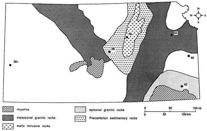
Figure 23--Plot of heat flow versus heat generation for the midcontinent. Line and data from Levasy, Missouri, and Picher, Oklahoma, are from Roy et al. (1968).
It might be anticipated that somewhat lower heat-flow values would be observed over the midcontinent gravity feature which runs through central Kansas. The hole in SW SW SW sec. 32, T. 13 S., R. 2 W., is close to this feature; however, the heat flow in that hole does not appear to be significantly below those observed in the other drill holes. Additional studies could allow investigation of the Precambrian basement more directly than has been possible in the past because of the relationship between surface heat flow and basement heat generation. Further detailed studies in holes, which do not penetrate basement rock, could be carried out in order to investigate the differences in heat flow and, therefore, the variations in basement geology. This technique would be of particular use in areas where the basement is too deep to be reached by many drill holes so that basement data are sparse.
A number of new techniques and/or modifications of existing techniques have been applied to evaluate the geothermal data from Kansas. The available data for four of the holes included a detailed temperature log for a major portion of the sedimentary section, several kinds of geophysical-well logs, a geological analysis of the cuttings, and the cutting samples themselves. As a result, we have been able to evaluate a number of new techniques and to apply these new techniques to increase the information that can be obtained from the relatively small number of holes available.
Correlation of the geothermal-gradient data with the well-logging data allowed recognition of errors apparently existing in previous determinations of shale thermal-conductivity values which, in turn, caused some errors in estimates of heat flow in the midcontinent region.
Results demonstrate that the contrast in thermal conductivity between limestone and shale may reach 2.5:1, and the conductivity contrast between shale and dolomite or evaporite deposits may approach 1:4. Using the well-log data, we have demonstrated that there is no significant variation in heat flow down the length of the boreholes so that the contribution in the surface-heat flow from any flow in such aquifers as the Arbuckle Group must be less than 5 mWm-2.
Steele et al. (1981) presented the preliminary results of this research and described the problems with literature values of shale thermal conductivity. The point was amplified and discussed in more detail by Blackwell and Steele (1988). Subsequent to the initial report, Sass and Galanis (1983) studied in detail the thermal conductivity of a sample of the Cretaceous-age Pierre Shale from a core hole near Hayes, South Dakota. The sample had been preserved in as near in situ conditions as possible. They obtained a value for the vertical component of thermal conductivity of 1.19 ± 0.05 Wm-1K-1 and a value for the horizontal component of thermal conductivity of 1.38 ± 0.04 Wm-1K-1. These values are consistent with values inferred for shales in this study. A further implication is that shales must show a modest compaction effect on thermal conductivity if dense lower Paleozoic shales have similar thermal conductivity values to Upper Cretaceous shale (see Blackwell and Steele, 1988).
Recently Gosnold (1985, 1989) has documented the effect of regional aquifer motions on surface heat flow in the Dakotas and Nebraska. The results of this study indicate that these types of effects do not influence the heat flow in central and eastern Kansas. In the area of this study, heat flow is constant to within a few meters of the basement surface. Regional fluid flow may be present in the Cenozoic and Mesozoic aquifers in western Kansas outside the area of this report, however.
The geothermal potential of a particular area depends on a number of different factors. In Kansas, the use of geothermal energy will be restricted to lower temperature applications such as heat pumps, thermal assist, and perhaps some direct space heating. In spite of the rather thin sedimentary section, relatively high temperatures apparently exist in the sediments. The temperature map in fig. 12 shows an estimate of these temperatures at a depth of 500 m (1,650 ft). The lateral and vertical temperature variations will depend primarily on three factors: heat production of basement rocks, presence or absence of slight disturbances of heat flow by aquifer motions, and lithological variations. Based on data discussed in this report, the second possible effect on heat flow and temperature variation seems to be minor, at least in the eastern half of the state, even though geothermal gradients vary drastically between the upper and lower parts of several of the holes. The analysis indicates that the heat-flow values do not vary because the thermal conductivity offsets the variations in gradient. No evidence exists for large-scale lateral transfer of heat in any of the possible aquifer systems that might exceed 10% of the surface-heat flow. Perhaps in western Kansas the water-flow effect could be more important, although this hypothesis cannot be accepted without proof.
The second major contributor to variation in temperature is the heat flow, primarily related to the heat production of the basement rocks. At the present time we have very little information on the distribution of heat production in the basement of Kansas. It will be valuable to make a systematic study of all existing core and cutting samples of the basement to determine the uranium, thorium, and potassium contents and to begin a preliminary evaluation of the heat-production distribution in the basement. This study will allow a relatively precise estimate of the heat flow at any prospective geothermal-use site based on the relationship between heat flow and heat production shown in fig. 23.
The third and possibly most significant contribution to the temperature at depth is the total thermal resistance of the section from the surface to that particular depth, i.e. the distribution of thermal conductivity with depth. Several of these holes illustrate the extreme differences in geothermal gradient related to thermal-conductivity contrasts. One clear conclusion from the results of this study is that in evaluating the temperatures at a particular depth, simple extrapolation of observed data from over one depth to a greater depth is not justified without consideration of the intervening lithology. It has been demonstrated in this paper that good estimates of the mean thermal resistance of the Pennsylvanian and older geologic sections can be obtained from well-log data. Utilizing available well-log information, the thermal resistance of the sedimentary section can be estimated, and areas can be selected for temperature logging which have the highest probability of high temperatures. The same techniques can be used to evaluate the probable temperature at depth near areas where utilization of the geothermal resource might be contemplated.
In the past few years, much attention has been focused on the eastern United States to evaluate geothermal potential. The evaluation has been based on the concept that radiogenic plutons underlie low thermal-conductivity Mesozoic and Cenozoic sedimentary rocks with projected temperatures of 40-60°C (104-140°F) maximum (Costain et al., 1977). Recognition that the high gradients observed in areas of the midcontinent are related to a much lower thermal conductivity than previously has been realized suggests that the radiogenic-pluton concept can be applied to the midcontinent region as well as to the eastern United States. Even though the age of most of the rocks in the midcontinent is Paleozoic to Mesozoic, the thermal conductivities of the shales do not seem to be any higher; in fact, they may be lower than typical values of similar units of Cenozoic age. Therefore, regions of the midcontinent with relatively thick shale sections have as high or higher geothermal gradients for a given heat flow than those observed in the Atlantic coastal-plain region. Thus, exploration for high-radioactive plutons in the midcontinent could identify numerous areas of greater potential geothermal energy than previously have been expected. In some of the deep basins in the midcontinent, thicker sections of sedimentary rocks are available than in the eastern United States. For example, the thick Devonian shales of the Appalachian region and the thick Cretaceous shales of the Great Plains cause very high temperatures to be observed at relatively moderate depths (Gosnold, 1985, 1989). Evaluation of basement rocks of the midcontinent and the location of potential geothermal targets using gravity, magnetic, and temperature data should outline targets more favorable for geothermal energy than those presently outlined in the eastern United States. For example, if a large region of the basement has a heat generation similar to the White Mountain batholith of New England (6 mWm-3), the predicted heat flow would be about 85 mWm-2, and the typical gradients in sections of shale such as those in Kansas would be approximately 70°C/km.
In spite of its location in the Central Stable Region, some areas of the state of Kansas have temperatures high enough to be used as thermal assistance for space heating and perhaps for direct space heating. These temperatures are available in the sedimentary section where possible aquifers exist for production of the required fluid. Additional work could more clearly outline areas of given temperature (in particular, aquifers) so that the total geothermal potential can be determined.
This paper was submitted in essentially the present form as a technical report for a subcontract from the Kansas Geological Survey in 1981. Updated results were presented at the Kansas geophysics symposium in 1985. This study could not have been completed without the interest and encouragement of Don Steeples and his contribution is gratefully acknowledged.
Bickford, M. E., Harrower, K. L., Nusbaum, R. L., Thomas, J. J., and Nelson, G. E., 1979, Geologic map of the Precambrian basement rocks of Kansas: Kansas Geological Survey, Map M-9, scale 1:500,000.
Birch, F., 1947, Crustal structure and surface-heat flow near the Colorado front range: American Geophysical Union, Transactions, 28, p. 792-797.
Blackwell, D. D., 1969, Heat flow determinations in the northwestern United States: Journal of Geophysical Research, 74, p. 922-1,007.
Blackwell, D. D., 1978, Heat flow and energy loss in the western United States; in, Cenozoic Tectonics and Regional Geophysics of the Western Cordillera, R. B. Smith and G. P. Eaton, eds.: Geological Society of America, Memoir 152, p. 175-203.
Blackwell, D. D., and Spafford, R. E., 1987, Experimental methods in continental heat flow; in, Experimental Methods in Physics, v. 24--Geophysics, Part B-Field Measurements, C. G. Sammis and T. L. Henyey, eds.: Academic Press, p. 189-226.
Blackwell, D. D., and Steele, J. L., 1988, Thermal conductivity of sedimentary rock-measurement and significance; in, Thermal History of Sedimentary Basins-Methods and Case Histories, N. D. Naeser and Th. H. McCulloh, eds.: Springer-Verlag, p. 13-36.
Combs, J., and Simmons, G., 1973, Terrestrial heat-flow determinations in the north-central United States: Journal of Geophysical Research, v. 78, p. 441-461.
Constain, J. K., Glover, L. III, and Sinha, A. K., 1977, Evaluation and targeting of geothermal-energy resources in the southeastern United States: U.S. Department of Energy, Report VPI-SU-5648-1.
Decker, E. R., and Roy, R. F., 1974, Basic heat-flow data from the eastern and western United States; in, Basic Heat-Flow Data from the United States, J. H. Sass and R. J. Munroe, comp: U.S. Geological Survey, Open-file Report 74-9, p. 7-1 to 7-89.
Garland, G. D., and Lennox, D. H., 1962, Heat flow in western Canada: Geophysical Journal of the Royal Astronomical Society, v. 6, p. 245-262.
Gosnold, W. D., Jr., 1989, Heat flow in the Great Plains of the United States: Journal of Geophysical Research, in press.
Gosnold, W. D., Jr., 1985, Heat flow and ground-water flow in the Great Plains of the United States: Journal of Geodynamics, v. 4, p. 247-264.
Gosnold, W. D., Jr., 1976, A model for uranium and thorium assimilation by intrusive magmas and crystallizing plutons through interaction with crustal fluids: Ph.D. dissertation, Southern Methodist University, 131 p.
Gosnold, W. D., Jr., and Eversoll, D. A., 1982, Geothermal resources of Nebraska: Boulder, Colorado, National Geophysical and Solar-Terrestrial Data Center, map scale 1:500,000.
Goss, R. and Combs, J., 1976, Thermal-conductivity measurement and prediction from geophysical well-log parameters with borehole application: Proceedings of 2nd U.N. Symposium on Geothermal Energy, U.S. Government Printing Office, Washington, D.C., p. 1,019-1,027.
Judge, A. S., and Beck, A. E., 1973, Analysis of heat-flow data--several boreholes in a sedimentary basin: Canadian Journal of Earth Science, 10, p. 1,494-1,507.
Lachenbruch, A. H., and Sass, J. H., 1977, Heat flow in the United States and the thermal regime of the crust; in, The Earth's Crust, J. G. Heacock, ed: American Geophysical Union, Geophysical Monograph 20, p. 626-675.
Robertson, E. C., 1975 (1988), Thermal properties of rocks: U.S. Geological Survey, Open-file Report, 88-441, 106 p. [available online]
Roy, R. F., Blackwell, D. D., and Birch, F., 1968, Heat generation of plutonic rocks and continental heat-flow provinces: Earth and Planetary Science Letters, v. 5, p. 1-12.
Roy, R. F., Decker, E. R., Blackwell, D. D., and Birch, F., 1968,Heat flow in the United States: Journal of Geophysical Research, v . 73, p. 5,207-5,221.
Sass, J. H., and Galanis, S. P., Jr., 1983, Temperatures, thermal conductivity, and heat flow from a well in Pierre Shale near Hayes, South Dakota: U.S. Geological Survey, Open-file Report 83-25, 10 p. [available online]
Sass, J. H., Lachenbruch, A. H., and Munroe, R. S., 1971, Thermal conductivity of rocks from measurements on fragments and its application to heat-flow determinations: Journal of Geophysical Research, v. 76, p. 3,391-3,401.
Sass, J. H., Lachenbruch, A. H., Munroe, R. J., Greene, G. W., and Moses, T. H., Jr., 1971, Heat flow in the western United States: Journal of Geophysical Research, v. 76, p. 6,356-6,431.
Scattolini, R., 1978, Heat-flow and heat-production studies in North Dakota: Ph.D. dissertation, University of North Dakota, 264 p.
Steele, J. L, Blackwell, D. D., and Steeples, D. W., 1981, Heat-flow determinations in Kansas and their implications for midcontinent heat-flow patterns: EOS, Transactions of the American Geophysical Union, v. 62, p. 392.
Swanberg, C. A., and Morgan, P., 1979, The linear relation between temperatures based on the silica content of ground water and regional heat flow-a new heat flow map of the United States: Pure and Applied Geophysics, v. 117, no. 1, p. 227-241.
Williams, J., 1981, Prediction of thermal-conductivity values from well logs and laboratory measurements of velocity with application to geothermal test well INEL-GT1: M.S. thesis, Southem Methodist University.
| Smoky Hill, Kansas, SW SW SW sec. 32, T. 13 S., R. 2 W. | |
|---|---|
| Depth (ft) |
Bulk conductivity Wm-1K-1 |
| 950-960 | 3.39 |
| 906-970 | 3.64 |
| 1,700-1,710 | 2.70 |
| 1,750-1,760 | 3.22 |
| 1,860-1,870 | 2.80 |
| 1,940-1,950 | 2.82 |
| 2,010-2,020 | 2.62 |
| 2,100-2,110 | 2.96 |
| 2,150-2,160 | 2.98 |
| 2,260-2,270 | 2.74 |
| 2,350-2,360 | 2.98 |
| 2,440-2,450 | 2.62 |
| 2,560-2,570 | 2.68 |
| 2,650-2,660 | 3.04 |
| 2,700-2,710 | 3.86 |
| 2,760-2,770 | 4.21 |
| 2,860-2,870 | 2.65 |
| 2,950-2,960 | 2.54 |
| 3,020-3,030 | 3.84 |
| 3,070-3,080 | 3.26 |
| 3,130-3,140 | 3.28 |
| 3,150-3,160 | 2.82 |
| 3,210-3,220 | 2.77 |
| 3,250-3,260 | 3.12 |
| 3,345-3,355 | 2.97 |
| 3,400-3,410 | (2.31) |
| 3,446-3,456 | 3.72 |
| 3,500-3,510 | 4.53 |
| 3,550-3,560 | 4.35 |
| 3,600-3,610 | 3.90 |
| 3,650-3,660 | 4.97 |
| Watson-1, Kansas, SE SW SE sec. 18, T. 18 S., R. 23 E. | |
|---|---|
| Depth (ft) |
Bulk conductivity Wm-1K-1 |
| 350-355 | 4.11 |
| 405-410 | 2.72 |
| 450-455 | 2.89 |
| 505-510 | 2.92 |
| 550-555 | 2.41 |
| 600-605 | 2.52 |
| 650-655 | 2.98 |
| 700-705 | 2.63 |
| 755-760 | 2.78 |
| 770-775 | 3.02 |
| 820-825 | 3.23 |
| 850-855 | 2.40 |
| 895-900 | 2.90 |
| 945-950 | 3.21 |
| 995-1,000 | 4.46 |
| 1,050-1,055 | 3.12 |
| 1,105-1,110 | 3.69 |
| 1,150-1,155 | 3.95 |
| 1,200-1,205 | 2.28 |
| 1,210-1,215 | 2.96 |
| 1,250-1,255 | 3.85 |
| 1,355-1,360 | 4.82 |
| 1,450-1,455 | 4.50 |
| 1,550-1,555 | 4.85 |
| 1,650-1,655 | 4.38 |
| 1,745-1,750 | 5.13 |
| 1,855-1,860 | 5.29 |
| Big Springs, Kansas, NW NW SE sec. 13, T. 12 S., R. 17 E. | |
|---|---|
| Depth (ft) |
Bulk conductivity Wm-1K-1 |
| 300-310 | 2.71 |
| 400-410 | 2.76 |
| 500-510 | 3.49 |
| 550-560 | 2.47 |
| 570-580 | 2.53 |
| 600-610 | 2.69 |
| 700-710 | 2.39 |
| 750-760 | 2.86 |
| 800-810 | 2.33 |
| 840-850 | 2.77 |
| 890-900 | 2.69 |
| 900-910 | 2.81 |
| 910-920 | 3.19 |
| 920-930 | 3.16 |
| 930-940 | 2.68 |
| 940-950 | 2.80 |
| 960-970 | 3.16 |
| 1,000-1,010 | 3.03 |
| 1,100-1,110 | 2.63 |
| 1,200-1,210 | 2.26 |
| 1,300-1,310 | 2.41 |
| 1,400-1,410 | 2.39 |
| 1,490-1,500 | 2.67 |
| 1,500-1,510 | 3.28 |
| 1,520-1,530 | 3.61 |
| 1,530-1,540 | 3.10 |
| 1,560-1,570 | 3.12 |
| 1,580-1,590 | 2.66 |
| 1,600-1,610 | 4.76 |
| 1,620-1,630 | 3.86 |
| 1,640-1,650 | 3.28 |
| 1,660-1,670 | 2.94 |
| 1,680-1,690 | 2.92 |
| 1,690-1,700 | 2.62 |
| 1,700-1,710 | 3.14 |
| 1,710-1,720 | 3.21 |
| 1,720-1,730 | 3.26 |
| 1,740-1,750 | 3.23 |
| 1,760-1,770 | 3.11 |
| 1,780-1,790 | 3.11 |
| 1,800-1,810 | 3.05 |
| 1,810-1,820 | 3.48 |
| 1,820-1,830 | 3.48 |
| 1,900-1,910 | 2.79 |
| 1,990-2,000 | 2.93 |
| 2,000-2,010 | 3.04 |
| 2,050-2,060 | 2.51 |
| 2,080-2,090 | 2.45 |
| 2,100-2,110 | 2.48 |
| 2,150-2,160 | 4.82 |
| 2,200-2,210 | 4.11 |
| 2,250-2,260 | 5.02 |
| 2,300-2,310 | 4.66 |
| 2,350-2,360 | 5.46 |
| 2,400-2,410 | 4.06 |
| 2,450-2,460 | 5.07 |
| 2,500-2,510 | 3.93 |
| 2,550-2,560 | 5.67 |
| 2,600-2,610 | 5.03 |
| 2,650-2,660 | 5.48 |
| 2,700-2,710 | 4.36 |
| 2,750-2,760 | 5.09 |
| 2,800-2,810 | 4.66 |
| 2,850-2,860 | 6.10 |
| 2,900-2,910 | 4.69 |
| 2,950-2,960 | 3.94 |
| U.S. Geological Survey Big Springs, SW NE SW sec. 22, T. 31 S., R. 20 E. |
|
|---|---|
| Depth (ft) |
Bulk conductivity Wm-1K-1 |
| 230-240 | 2.99 |
| 280-290 | 2.88 |
| 330-340 | 2.78 |
| 380-390 | 2.88 |
| 430-440 | 2.66 |
| 480-490 | 2.46 |
| 530-540 | 2.41 |
| 580-590 | 2.78 |
| 630-640 | 3.17 |
| 670-680 | 2.26 |
| 680-690 | 2.50 |
| 690-700 | 2.35 |
| 700-710 | 2.74 |
| 710-720 | 2.69 |
| 730-740 | 4.09 |
| 745-750 | 4.62 |
| 770-775 | 6.16 |
| 795-800 | 4.43 |
| 850-855 | 3.61 |
| 905-910 | 4.95 |
| 950-955 | 4.39 |
| 1,000-1,005 | 5.43 |
| 1,050-1,055 | 5.13 |
| 1,100-1,105 | 4.85 |
| 1,145-1,150 | 5.25 |
| 1,200-1,210 | 5.58 |
| 1,250-1,255 | 6.33 |
| 1,300-1,305 | 5.11 |
| 1,350-1,355 | 5.14 |
| 1,400-1,405 | 5.14 |
| 1,445-1,450 | 5.53 |
| 1,495-1,500 | 5.80 |
| 1,545-1,550 | 5.36 |
| 1,600-1,605 | 5.05 |
| 1,650-1,655 | 5.92 |
| 1,700-1,705 | 5.18 |
| 1,750-1,760 | 5.06 |
| 1,800-1,805 | 4.97 |
| Core Conductivity | Wm-1K-1 |
| 2,968' 8" - 2,968' 9" | 3.22 |
| 2,970' 5" - 2,970' 6" | 3.21 |
| 2,974' 1.5" - 2,974' 2.5" | 3.22 |
| 2,977' 3" - 2,977' 4" | 3.22 |
Kansas Geological Survey
Comments to webadmin@kgs.ku.edu
Web version Sept. 16, 2013. Original publication date 1989.
URL=http://www.kgs.ku.edu/Publications/Bulletins/226/Blackwell/index.html