Kansas Geological Survey, Bulletin 211, Part 4, p. 10-16
Public Law 92-500, the Federal Water Pollution Control Act, particularly Section 102, mandates the Environmental Protection Agency to "prepare or develop comprehensive programs for preventing, reducing, or eliminating the pollution of the navigable waters and groundwaters and improving the sanitary condition of surface and underground waters." These investigations have necessitated the development of a groundwater quality graphic display for use in planning, management, and control processes.
The efficiency of a graphic has long been known; witness the ancient Chinese proverb "A picture is worth a thousand words." There are several components to this efficiency. A good diagram is simple and speedily read; if used more than once it is standardized, and hence comparable. Simplicity is achieved by keeping the information content to a workable level, which for most readers is seven ± two bits of information. This simplicity in turn promotes quick understanding. Standardization of format of a diagram is a must if this diagram is to be used for the comparison and analysis of data. But perhaps the most important feature of a graphic is that it allows an observer to see a pattern which might well have remained obscure if the information were left in some other form. Robinson and Petchenik (1976) say it more succinctly. "Structures are likely to remain hidden until they have been mapped." Anyone who has been confronted by a set of apparently unrelated numbers (Table 1) will appreciate the simplicity and beauty of a well-designed diagram (Fig. 1).
Table 1--Selected well records for Scott and Lane counties, in western Kansas. (Data from Hathaway et al., 1975.)
| Well Number |
Well Location |
Date of Collection |
SiO2 ppm |
Ca ppm |
Mg ppm |
Na ppm |
K ppm |
HCO3 ppm |
SO4 ppm |
Cl ppm |
F ppm |
NO4 ppm |
Total PO4 ppm |
|---|---|---|---|---|---|---|---|---|---|---|---|---|---|
| Scott County | |||||||||||||
| 31 | 16-31W-31BCB | 7/30/1974 | 55 | 69 | 25 | 26 | 6.0 | 207 | 76 | 42 | 2.3 | 26 | |
| 32 | 16-33W-6CCC | 8/1/1974 | 35 | 52 | 19 | 29 | 5.4 | 196 | 41 | 30 | 2.0 | 17 | .21 |
| 35b | 16-33W-25BCC | 8/1/1974 | 34 | 44 | 17 | 30 | 5.0 | 200 | 37 | 9.6 | 2.2 | 13 | |
| 38 | 16-34W-29CBB | 7/31/1974 | 25 | 43 | 18 | 29 | 4.9 | 205 | 47 | 10.4 | 1.7 | 15 | |
| 40 | 17-31W-31BBB | 7/31/1974 | 59 | 80 | 35 | 34 | 7.9 | 234 | 114 | 62 | 2.1 | 32 | |
| 43 | 17-32W-31BCB | 7/30/1974 | 58 | 55 | 24 | 31 | 6.2 | 207 | 63 | 34 | 2.6 | 23 | |
| 48 | 17-34W-6BCB | 7/31/1974 | 26 | 42 | 15 | 30 | 4.9 | 209 | 42 | 9.9 | 1.7 | 13 | |
| 53 | 18-33W-3CCB | 7/30/1974 | 60 | 44 | 22 | 30 | 5.6 | 208 | 54 | 20 | 2.4 | 15 | |
| 58 | 18-34W-30DDC | 7/31/1974 | 52 | 56 | 22 | 30 | 6.2 | 222 | 53 | 28 | 1.8 | 18 | |
| 60d | 19-31W-20BAD | 8/1/1974 | 29 | 86 | 14 | 28 | 7.6 | 262 | 47 | 45 | .6 | 22 | |
| 62c | 19-33W-24ABB | 7/31/1974 | 37 | 125 | 71 | 107 | 10.8 | 312 | 483 | 65 | 2.1 | 15 | .01 |
| Lane County | |||||||||||||
| 21 | 16-29W-26CCD | 8/1/1974 | 52 | 53 | 21 | 20 | 5.5 | 227 | 39 | 17 | 2.3 | 12 | .19 |
| 22 | 16-30W-24DCC | 8/1/1974 | 48 | 52 | 21 | 23 | 5.6 | 216 | 43 | 19 | 2.3 | 16 | |
| 27 | 17-29W-36BAA | 8/1/1974 | 51 | 53 | 24 | 30 | 6.8 | 244 | 59 | 19 | 3.1 | 12 | |
| 29 | 18-29W-4DAD | 8/1/1974 | 56 | 65 | 33 | 28 | 7.9 | 245 | 78 | 49 | 4.6 | 9 | .18 |
| 30 | 18-30W-2AAA | 8/1/1974 | 57 | 71 | 33 | 41 | 8.3 | 242 | 155 | 32 | 3.1 | 15 | |
| Well Number |
Well Location |
Date of Collection |
Fe ppb |
Mn ppb |
Sr ppm |
Ni ppb |
Zn ppb |
Temp. °C |
Total Dis. Solids 180°C |
Hardness as CaCO3 |
Specific Conductance (micromhos at 25°C) |
SAR | pH | |
|---|---|---|---|---|---|---|---|---|---|---|---|---|---|---|
| Total ppm |
Non- Carbonate ppm |
|||||||||||||
| Scott County | ||||||||||||||
| 31 | 16-31W-31BCB | 7/30/1974 | 7 | 2 | 1.2 | 3 | 4 | 16.5 | 425 | 277 | 107 | 695 | .68 | 7.3 |
| 32 | 16-33W-6CCC | 8/1/1974 | 8 | 1 | 1.0 | 1 | 4 | 16.5 | 343 | 211 | 50 | 470 | .87 | 7.7 |
| 35b | 16-33W-25BCC | 8/1/1974 | 4 | 2 | .9 | 2 | 4 | 15.5 | 314 | 180 | 16 | 480 | .97 | 6.8 |
| 38 | 16-34W-29CBB | 7/31/1974 | 13 | 2 | .8 | 4 | 24 | 15.5 | 294 | 183 | 15 | 400 | .93 | 7.2 |
| 40 | 17-31W-31BBB | 7/31/1974 | 8 | 2 | 1.7 | 5 | 4 | 16.0 | 438 | 347 | 155 | 830 | .79 | 7.3 |
| 43 | 17-32W-31BCB | 7/30/1974 | 11 | 3 | 1.1 | 2 | 24 | 16.0 | 407 | 238 | 68 | 600 | .87 | 6.9 |
| 48 | 17-34W-6BCB | 7/31/1974 | 17 | 2 | .8 | 4 | 3 | 17.0 | 291 | 167 | 0 | 590 | 1.01 | 7.6 |
| 53 | 18-33W-3CCB | 7/30/1974 | 34 | 2 | 1.1 | 3 | 12 | 17.0 | 352 | 201 | 30 | 762 | .92 | 6.8 |
| 58 | 18-34W-30DDC | 7/31/1974 | 26 | 3 | 1.2 | 6 | 12 | 16.5 | 384 | 234 | 52 | 589 | .85 | 6.8 |
| 60d | 19-31W-20BAD | 8/1/1974 | 15 | 2 | .6 | 3 | 8 | 15.0 | 404 | 272 | 57 | 687 | .74 | 7.0 |
| 62c | 19-33W-24ABB | 7/31/1974 | 32 | 10 | 3.5 | 83 | 8 | 17.5 | 1094 | 607 | 351 | 1510 | 1.89 | 7.2 |
| Lane County | ||||||||||||||
| 21 | 16-29W-26CCD | 8/1/1974 | 6 | 2 | 1.0 | 0 | 50 | 16.0 | 352 | 218 | 32 | 500 | .59 | 7.6 |
| 22 | 16-30W-24DCC | 8/1/1974 | 14 | 2 | 1.0 | 0 | 23 | 16.0 | 356 | 217 | 40 | 520 | .68 | 7.6 |
| 27 | 17-29W-36BAA | 8/1/1974 | 17 | 3 | .9 | 3 | 21 | 15.0 | 392 | 231 | 31 | 601 | .86 | 7.2 |
| 29 | 18-29W-4DAD | 8/1/1974 | 8 | 1 | 1.1 | 7 | 6 | 18.5 | 471 | 300 | 99 | 733 | .70 | 7.2 |
| 30 | 18-30W-2AAA | 8/1/1974 | 3 | 2 | 1.3 | 11 | 5 | 15.5 | 541 | 315 | 117 | 822 | 1.00 | 7.2 |
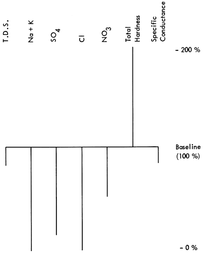
Figure 1--Baseline diagram from Scott Co., Kansas. Well #16 31W 31BCB.
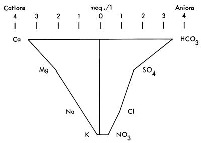
Hydrogeology, as a science, has long used diagrams to display groundwater information to assist understanding chemical analyses (Hem, 1959). One of the most frequently used quantitative graphics is the Stiff Pattern (Fig. 2). This display shows cations versus anions radiating from a central spine. The outlying points are then connected by a circumscribing line. The resulting pattern can be compared with other Stiff patterns to ascertain if similarities exist between samples (Stiff, 1951).
Figure 2--Stiff diagram from Scott Co., Kansas. Well #16 31W 31BCB.
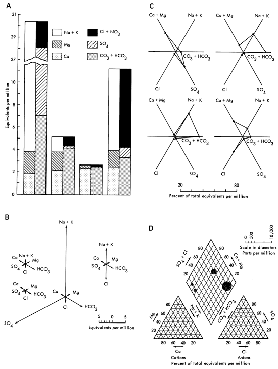
Other diagrams in use are Collin's vertical bar graphs, Mancha's radiating vectors, Tickell's radial coordinates, and Piper's tri-linear, examples of which will be found in Fig. 3a-d. These graphics all suffer from several disadvantages. They are difficult to interpret, slow to read, and time consuming to construct. These diagrams are used by chemists and hydrologists in a quantitative way, and as such, have two drawbacks when used to discuss groundwater quality. The first is that these displays have little or no qualitative information for the observer. For instance "Are 80 milliequivalents/ liter (meq/l) of calcium good or bad?" If it is good, "Is it twice as good as having 160 meq/l of calcium?" These questions face one when working with conventional chemical analysis diagrams. The second problem is really the other side of the coin. An untrained observer will not only not know "How much is good?", but frequently will not know about the existence of anions or cations. As can be seen, conventional diagrams have some shortcomings.
Figure 3--Some popular hydrologic diagrams (from Hem, 1959); A. Collin's vertical bar graphs; B. Maucha's radiating vectors; C. Tickell's radial coordinates; D. Piper's tri-linear.
It would seem then to be an advantage to have a graphic which would not only show quantitative chemical content but also would give a qualitative indication of the water sample. With the development of the Baseline Diagram (Fig. 1), this is now possible. The concept of a non-zero baseline is important as it allows us to depict any deviation from an accepted norm, and tell if something is "good" or "bad" relative to that norm.
The baseline is constructed from the maximum acceptable values of some groundwater quality criteria which are reported in a standard water quality chemical analysis. The value of a non-zero baseline is that it not only allows depiction of the chemical constituents of a water sample, it also allows the observer to make a quality judgment about the water quality relative to the baseline standard. The above and below baseline scaling is predicated on the basis that the baseline represents 100%, of the acceptable level of chemical constituents, and that any deviation is some percentage of the baseline value. The scaling is shown in Table 2.
Table 2--Scaling factors for the Baseline Diagram.
| TDS mg/l |
Na+K mg/l |
SO4 mg/l |
Cl mg/l |
NO3 mg/l |
Total Hardness mg/l |
Specific Conductance µmhos/cm |
||
|---|---|---|---|---|---|---|---|---|
| 1500 | 600 | 750 | 750 | 135 | 450 | 2250 | 300% | |
| 1400 | 560 | 700 | 700 | 126 | 420 | 2100 | ||
| 1300 | 520 | 650 | 650 | 117 | 390 | 1950 | ||
| 1200 | 480 | 600 | 600 | 108 | 360 | 1800 | ||
| 1100 | 440 | 550 | 550 | 99 | 330 | 1650 | ||
| 1000 | 400 | 500 | 500 | 90 | 300 | 1500 | 200% | |
| 900 | 360 | 450 | 450 | 81 | 270 | 1350 | ||
| 800 | 320 | 400 | 400 | 72 | 240 | 1200 | ||
| 700 | 280 | 350 | 350 | 63 | 210 | 1050 | ||
| 600 | 240 | 300 | 300 | 54 | 180 | 900 | ||
| Baseline | 500 | 200 | 250 | 250 | 45 | 150 | 750 | 100% |
| 400 | 160 | 200 | 200 | 36 | 120 | 600 | ||
| 300 | 120 | 150 | 150 | 27 | 90 | 450 | ||
| 200 | 80 | 100 | 100 | 18 | 60 | 300 | ||
| 100 | 40 | 50 | 50 | 9 | 30 | 150 | ||
| 0 | 0 | 0 | 0 | 0 | 0 | 0 | 0% |
The seven criteria (Table 3) were chosen because they are readily available from chemical analyses and they communicate water quality information to the untrained as well as the trained observer. Following are the seven constituents and the logic for their selection:
T.D.S. content is a general indication of water quality, as it reflects the qualitity of inorganic salts, dissolved material, and small amounts of organic matter (Sawyer, 1960) left in solution. Generally the higher the T.D.S., the poorer the water quality. According to Sawyer (1960), this measure is associated with unpalatable mineral tastes, possible physiological effects, and high costs due to corrosion.
High sodium can have a deleterious health effect on people who are on a restricted sodium diet, as is the case with some heart patients. Excess sodium, in conjunction with high chlorides, may indicate intrusion of brine into an aquifer or subsurface water body. (In some chemical analyses these two components, sodium and potassium, are reported already summed.)
Since chloride will readily combine with different cations to produce several different salts, this chemical is an indicator of the presence of brine and other salts as well as the potential for salinity in groundwater.
This anion occurs naturally in small quantities in surface and groundwater (0 to 100 mg/l), but more often is the result of industrial discharges. Sulphate salts of magnesium and sodium are noted for having a laxative effect on humans if amounts greater than 250 mg/l are found in drinking water.
This has been shown to be the cause of poisoning in young infants (methemoglobinemia) where the nitrogen concentration in drinking water is 10 mg/l or more. High nitrates are also generally associated with high bacteria counts, such as one would find with effluent intrusion into the groundwater from sources such as feedlots, septic-tank leakage, or sanitary landfills.
This is a general measure, the greater part of which is usually carbonate hardness. Although not usually a health problem, carbonate waters can be an economic problem as they tend to cause buildup of scale in pipes and valves necessitating expensive repair or replacement.
Conductance is a measure of the concentration of soluble salts, and as such is used to gauge the acceptability of irrigation water. "In general, waters with conductivity values below 750 mhos/cm are satisfactory for irrigation, although salt sensitive crops may be adversely affected by conductivity values in the 250 to 750 mhos/cm range" (U.S. Salinity Laboratory, 1951). Conductance is also a readily available field test which enables a worker to compare a new sample with previously analyzed samples quickly and easily.
Although one could choose other criteria, these seem to give an accurate picture of groundwater quality as it relates to the several areas of potential health hazards, industrial pollution, and irrigation hazards.
Table 3--Baseline criteria, values and authority for selection. Federal law mandates the maximum contaminant level of Nitrate (NO3) as Nitrogen (N) to be 10 mg/l (EPA 570/9-76-003), but because chemical analyses report Nitrate as NO3 and not N, a conversion must be made. The factor 4.4268, when multiplied by a quantity of N will yield an equivalent quantity of NO3 (Lange, 1967). A maximum level of 10 mg/l of N will give a baseline level for NO3 of 44.268 mg/l, which is approximated by 45 mg/l.
| Criteria | Values | Authority |
|---|---|---|
| Total Dissolved Solids | 500 mg/l | EPA 440/9-76-023 |
| Sodium plus Potassium | 200 mg/l | EPA 440/9-76-023 |
| Siilpbate | 250 mg/l | EPA 440/9-76-023 |
| Chloride | 250 mg/l | EPA 440/9-76-023 |
| Nitrate | 450 mg/l | EPA 440/9-76-023 |
| Total Hardness | 150 mg/l | EPA 440/9-76-023 |
| Specific Conductance | 750 µmhos/cm | U.S. Salinity Lab. |
The Baseline Diagram is easily drawn using squared or graph paper, 0.1 inch squares being most suitable. Figures 4a-d show a method of construction which has been found useful at the Kansas Geological Survey.
Figure 4a-d--A method of construction used at the Kansas Geological Survey.
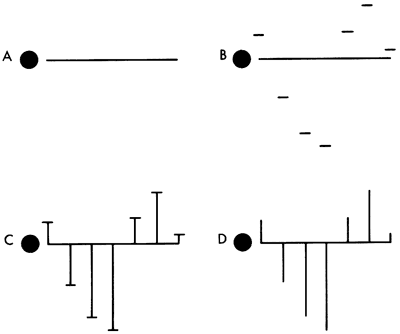
Figure 5 is a portion of a map of western Kansas using Stiff patterns to portray groundwater quality information. Figure 6 is the same area but utilizing instead the Baseline Diagram. As can be seen, the new graphic is better able to convey water-quality information to the reader by the simple observation, "the more bars below and the farther they are below the baseline the better the water."
Figure 5--Stiff patterns of selected wells in Scott and Lane counties, Kansas.
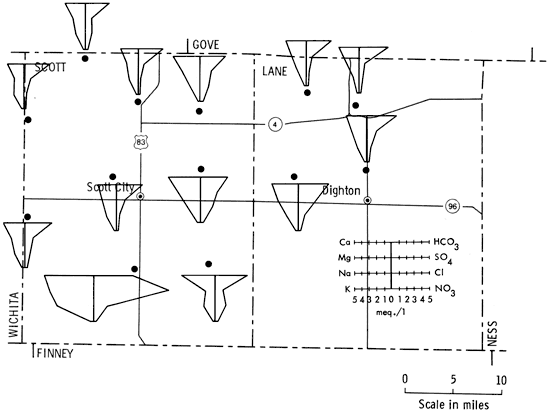
Figure 6--Baseline diagrams of selected wells in Scott and Lane counties, Kansas.
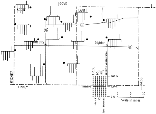
This new diagram would seem to have some advantages for use in groundwater analysis and reporting. It is speedily and easily read, yielding quality information to an untrained observer, i.e., the more bars and the higher they are above the line the poorer the water quality. It also allows quick comparison between the samples as there are three visual clues for pattern recognition: left to right sequence of bars, length of bars, and location and length of bars above or below the baseline. In short, this is a new tool for analyzing and displaying groundwater quality information quickly and efficiently.
Environmental Protection Agency, 1976, National Interim Primary Drinking Water Regulations. EPA # 570/9-76-003. C.P.O.: Washington, D.C.
Environmental Protection Agency, 1976a, Quality Criteria for Water. EPA # 440/9-76-023. G.P.O.: Washington, D.C.
Hathaway, L. R., Magnuson, L. M., Crr, B. L., Galle, O. K., and Waugh, T. C., 1975, Chemical Quality of Irrigation Waters in West-Central Kansas: Kansas Geol. Survey, Chemical Quality Series 2
Hem, John D., 1959, Study and Interpretation of the Chemical Characteristics of Natural Water. U.S. Geological Survey, Water Supply Paper 1473. G.P.O.: Washington, D.C.
Hernandez, John W., and Barkley, William A., 1976, The National Safe Water Drinking Act: New Mexico Water Resoures Research Institute, Report No. 071
Lange, J., 1967, Lange's Handbook of Chemistry, Revised 10th ed: McGraw Hill Book Co., Inc., New York
Robinson, Arthur H., and Petchenik, Barbara Bartz, 1976, The Nature of Maps: Univ. of Chicago Press, Chicago
Sawyer, C. H., 1960, Chemistry for Sanitary Engineers:. McGraw Hill Book Co., Inc., New York
Stiff, H. A., 1951, The Interpretation of Chemical Water Analysis by Means of Patterns: Journal of Petroleum Technology, v. 3, no. 10.
U.S. Salinity Laboratory, 1951, Diagnosis and Improvement of Saline and Alkali Soils: U.S. Dept. of Agriculture, Handbook No. 60, 160 pp.
U.S. Congress, 1972, Public Law 92-500: Federal Water Pollution Control Act Amendments of 1972: G.P.O., Washington
Kansas Geological Survey
Comments to webadmin@kgs.ku.edu
Web version updated June 18, 2010. Original publication date April 1978.
URL=http://www.kgs.ku.edu/Publications/Bulletins/211_4/dulas.html