Kansas Geological Survey, Bulletin 171, originally published in 1964
Prev Page--Start of Bulletin

Appendix A

Description of Computer Program for Fitting Four-variable Hypersurfaces

General Statement

Details of the computer program used in fitting. contouring, and evaluating four-variable trend hypersurfaces are presented in Appendix A. Appendix B is a complete listing of the computer program in which cards or lines are identified by number, and Appendix C consists of reproductions of examples of output from the program.

This program is written in a computer language called BALGOL, which is one of several "dialects" of the computer language termed ALGOL-58. A language such as BALGOL is termed a "source language." The program is placed initially on punched cards and then read into the computer where it is translated into machine language which the computer can utilize directly. The translation is accomplished by using another program, termed a compiler, which is usually recorded on magnetic tape and which translates, or compiles, the source language.

The program described here has been written primarily for use on either an IBM 7090 or 7094 computer, coupled with an IBM 1401 computer. The program could be used, with slight modifications, on the Burroughs 220 computer. The Kansas Geological Survey will make the program available, in punched-card form, for a limited time at a cost of $10.00. IBM 7090 and 7094 computers are currently in widespread use in the United States and access to one of these machines is available at a number of both university and commercial computer centers. Persons wishing to use the program on the IBM 7090 or 1094 should send four magnetic tapes to the Computation Center, Stanford University, Stanford, California, so that the BALGOL compiler system can be recorded on the tape. When this has been done, the program described in this report, as well as many other BALGOL programs, may be readily used on virtually any IBM 7090 or 7094 computer. Peter Carah wrote that part of the program for plotting of z values and residual values in the "slice maps," and the matrix inversion procedure was adapted from the Stanford University Computation Center program library.

The program is extremely fast and economical when run on the IBM 7090 or 7094 computer. The program compiles from the BALGOL source deck in 30 seconds. Time required for execution of the program varies, depending upon the number of data points and dimensions of the hypersurface blocks and plotted maps. As an example, 60 seconds 7090 time were required for execution using oil-gravity data described in this report, in which 244 data points were handled, three hypersurface blocks about 5 x 8 1/2 x 9 inches in dimensions were contoured, and 24 "slice maps" were plotted. In addition, about 6 minutes 1401 time were required for printing of the output.

Major Steps in Program

The theory and operation of the program are explained in detail on subsequent pages. However, as an introduction, the principal steps in the program are outlined below:

1. Read into computer numerical data that control certain operations of the program, such as dimensions of block contoured by computer.
2. Read in data values, four values (w, x, y, and z) for each data point.
3. Obtain sums for matrix and for column vector used in solution of normal equations.
4. Calculate constants of equations of hypersurfaces by matrix inversion.
5. Employing equation constants thus obtained, calculate trend value at each data point and subtract this value from actual z value at that point to obtain residual value. Each hypersurface of given degree will have its own trend and residual values at specified data points.
6. Calculate statistical properties of hypersurfaces, including error measure percent of total sum of squares, and apportionment of the sums of squares according to linear, quadratic, and abbreviated cubic components.
7. Calculate hypervolumes within hypersurfaces by evaluation of triple integral between limits of block. Divide hyper-volume by ordinary volume to obtain average value of z within block.
8. Contour intersections of hypersurface with planes that intersect block. The number of planes and their intersect values are specified on the control cards. Any number of horizontal and vertical planes may be contoured. It is generally convenient to contour the top, bottom, and four sides of the block whose limits have been specified in making previous calculations. Contouring is accomplished by substituting progressively changing values of w, x, or y corresponding to the location in space of each point for which a printed character is printed. Values of w, x, or y are substituted in equation describing surface, z value for each point is determined, and character to be printed (number, blank space, letter, or other symbol; Table 7) is selected, depending on value that z assumes at each point (Appendix C, Part 2).
9. If desired, the original data values and residual values from the three trend hypersurfaces are sorted according to depth and location and are then automatically plotted in a series of horizontal "slice maps" on which the values are plotted within specified depth intervals (Fig. 11, Appendix C, Part 3).

Input to Program

After the computer program has been fed into the computer, data cards follow. Three kinds of data cards are used in conjunction with this program: (1) alphabetical and numerical information used for identification purposes, (2) numerical information used to control the operation of the program, and (3) numerical values pertaining to data points. These data are described on subsequent pages. Detailed rules for preparation of data cards, as well as other information concerning BALGOL, are contained in the manual entitled Burroughs Algebraic Compiler: A Representation of ALGOL for Use with the Burroughs 220 Data-Processing System, which may be obtained from the Burroughs Corporation, Detroit, Michigan. The rules for data cards are very simple, however, and the most important are: (1) a 5 must be punched in column 1 of each data card, (2) columns 2 to 80 of each card are available for data, and (3) there is no specified format for the data values except that at least one blank column must separate numbers.

Alphanumeric heading. The first data consists of 72 characters of alphabetic and numerical (alphanumeric) information. Typically, this information might include the name of the area being studied, the name and age of the geologic formation or formations involved, and the name of the person preparing the data. When the program is executed, this information is reproduced at the top of each of the map pages (Appendix C) and elsewhere in the output pages, thus providing positive identification. Dollar signs should be placed in columns 2 and 75 of the data card, and the 72 alphanumeric characters (including blank spaces) are placed between the two dollar signs, in columns 3 to 74.

Control cards. (1) First control card:

1. A 5 in column 1 of each card.
2. An integer specifying whether the data point values are type integer (2222) or type decimal (4444).
3. An integer specifying the number of data points.
4. An integer specifying the length, in tenths of an inch, of the y dimension of the block that is to be contoured by the computer's printing machine. (Fig. 13).
5. An integer specifying the x dimension of the contoured block in tenths of an inch.
6. A decimal-point number specifying the x intercept of the right side of the block. The value must be expressed in x-coordinate units.
7. A decimal specifying the x intercept of left side of block.
8. A decimal specifying the y intercept of front of block. The value must be expressed in y-coordinate units.
9. A decimal specifying the y intercept in the back of block.
10. A decimal specifying the w intercept of bottom of block. The value must be expressed in w-coordinate units.
11. A decimal specifying the w intercept of top of block.
12. A decimal specifying the reference contour value.
13. A decimal specifying the contour interval.
14. An integer specifying the vertical, or w, dimension, in tenths of an inch, of the block that is to be contoured.
15. An integer specifying whether trend and residual values are to be written, written and punched, or neither written or punched as follows:
    0. Do not print or punch
    1. Print only
    2. Print and punch
16. An integer specifying whether raw data and residual values are to be plotted as follows:
    0. Do not plot
    1. Plot

(2) Second control card (for horizontal contoured surfaces):

1. A 5 in column 1.
2. An integer specifying the number of horizontal surfaces to be contoured; punch 0 if none are to be contoured.
3. Decimal numbers specifying intercept values of horizontal surfaces, expressed in w-axis coordinate units.

(3) Third control card (for vertical surfaces intersecting x axis)

1. A 5 in column 1.
2. An integer specifying the number of surfaces to be contoured; 0 if none are to be contoured.
3. Decimal numbers specifying x-axis intercept values of the surfaces.

(4) Fourth control card (for vertical surfaces intersecting y axis)

1. A 5 in column 1.
2. An integer specifying number of surfaces to be contoured; 0 if none are to be contoured.
3. Decimal numbers specifying y-axis intercept values of surfaces.

(5) Fifth control card (controls residual plotting; use only if integer specifying whether data values are to be plotted is 1 on first control card):

1. A 5 in column 1.
2. A decimal specifying the w intercept value of the top "slice" in which the original z values and residual values will be plotted. This number will have a smaller numerical value than in (d) below because the numbers increase going downward.
3. A decimal specifying the thickness in vertical (w-axis) units of each of the "slices."
4. A decimal specifying the w intercept value of the top of the bottom "slice." This number will necessarily be greater than the number in (b) above.

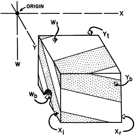
Figure 13--Diagram showing coordinate-axis intercept values (Xr, Xl, Yb, Yt, Wb, and Wt) for six planes that form surfaces of block intersecting hypersurface. (Intercept values must be in same units as w, x, and y values of data points.)

Values for data points. Four values for each data point are needed. These are fed in, in groups of four, in the order w, x, y, and z. The values may be either wholly decimal-point numbers or wholly integers, but may not be a mixture of both decimal and integer numbers. The w, x, and y values are coordinate values in arbitrary units, which may have a dimensional sense (feet, miles, fractions of inch, etc.), but could also represent any quantity that one wishes. For most geological purposes, it is convenient to express the w values in feet (well depth for example) and the x and y values in either miles or in fractions of an inch scaled from a map. The z values may be in any convenient units. If the integer on the first control card that specifies the type of data values is 2222, all values are to be in integer form, if 4444, all values in decimal-point numbers. Please note that a maximum of 950 data points may be handled without modification of the program. However, more data points could be handled by changing the array dimensions on lines 8, 12, and 19, Appendix B.

In obtaining the w-, x-, and y-coordinate values, it is most convenient to place the origin either at the upper left rear corner of the block or at some point that is farther to the left, higher, and farther to the rear. In a conventional geological application, the w-coordinate values might be well depths, with positive values that increase downward, and the x- and y-coordinate values might represent distances scaled from an origin along east-west and north-south directions, respectively. Negative values are acceptable. Cards are to be punched as follows:

1. (a) A 5 in column 1.
2. (b) w, x, y, and z values, in that order (any number of values per card, but numbers will be read in groups of four) .

Solutions of Normal Equations to Obtain Constants of Equations

Each hypersurface is described by an equation whose constants are such that the least-squares criterion is satisfied. The method employed involves matrix inversion and is basically the same for each hypersurface, regardless of the number of terms in its equation. For illustrative purposes, only the first-degree hypersurface is considered in detail

First-degree hypersurface. The equation for a first degree hypersurface is

z_trend = A + Bw + Cx + Dy      (Eq. A)

The constants A, B, C, and D of this equation are to be calculated so that the sum of the squared deviations is the least possible. The deviation at a particular point is that difference between the observed and calculated value, which may be expressed as

deviation = z_obs - z_trend

Because the ztrend value is given by equation A, we may rewrite equation as follows:

deviation = z_obs - (A + Bw + Cx + Dy) , or      (Eq. B)
deviation = z_obs - A - Bw - Cx - Dy

Proceeding further, we may express the sum of squared deviations as a function, F, of A, B, C, and D, by writing)

sum of squared deviations = F (A, B, C, D)      (Eq. C)

Combining equations B and C, we obtain

F (A, B, C, D) = Σ (z_obs - A - Bw - Cx - Dy )²

From this point on we will consider z to be z^obs.

If F (A, B, C, D) is to be minimized, it is necessary that

δF/δA = δF/δB = δF/δC = δF/δD = 0

The partial derivatives are

δF/δA = Σ 2(z - A - Bw - Cx - Dy) (-1) = 0
δF/δB = Σ 2(z - A - Bw - Cx - Dy) (-w) = 0
δF/δC = Σ 2(z - A - Bw - Cx - Dy) (-x) = 0
δF/δD = Σ 2(z - A - Bw - Cx - Dy) (-y) = 0

Multiplication of each expression and summation over the individual terms of these four equations yields four other equations, which are

-Σz + An + BΣw + CΣx + DΣy = 0
-Σzw + AΣw + BΣw² + cΣwx + DΣwy = 0
-Σzx + AΣx + BΣwx + CΣx² + DΣxy = 0
-Σzy + AΣy + BΣwy + CΣxy + DΣy² = 0

where n = number of data points.

We may rearrange these equations by placing the terms containing z on the other side to obtain four normal equations whose solution will permit us to obtain the four unknown constants, A, B, C, and D:

An + BΣw + CΣx + DΣy = Σz
AΣw + BΣw² + CΣwx + DΣwy = Σzw
AΣx + BΣwx + CΣx² + DΣxy = Σzx
AΣy + BΣwy + CΣxy + DΣy² = Σzy

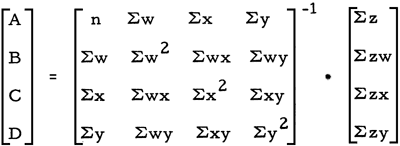
If a solution exists for these four linear equations, they may usually be solved by matrix algebra methods. We may restate the four normal equations by writing a single matrix equation, as follows:

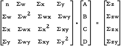
In this equation, the ABCD-vector multiplied by the wxy-matrix is equal to the vector containing z. In applying this equation, observational data provide the wxy-matrix and the z-vector, allowing the ABCD-vector to be determined. This may be done by multiplying the z-vector with the inverse of the wxy-matrix, so that

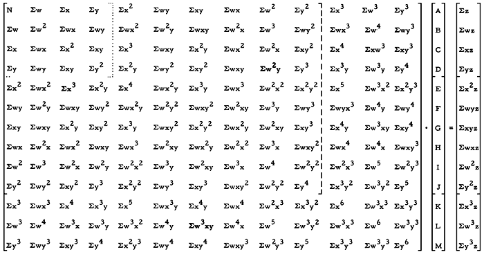
Second- and third-degree hypersurfaces. Second- and third-degree hypersurfaces are fitted in essentially the same manner as first-degree hypersurfaces, and the underlying theory is the same. There are more terms in the equations describing second- and third-degree surfaces, and therefore more normal equations are needed. The matrix equation for combined linear, quadratic, and part of the cubic terms is shown in Table 6. First-degree hypersurfaces involve only the linear terms (outlined by dotted lines in Table 6), second-degree hypersurfaces involve linear plus quadratic terms (outlined with dashed lines), and third-degree hypersurfaces involve all the linear plus quadratic plus cubic terms. It should be pointed out that the cubic terms are not complete in that the cubic cross-product terms have been arbitrarily omitted to cut down on the number of steps in the program.

Table 6--Matrix equation for obtaining constants of hypersurface equations. Left column vector contains constants A to M; Square matrix contains w, x, and y elements; right column vector contains w, x, y, and z elements. First-degree matrix equation is contained within dotted lines; second-degree matrix equation is contained within dashed lines (includes first-degree elements); abbreviated third-degree matrix equation contains all elements.

Steps in computer program in solving normal equations. The summation to obtain the values for z-vector and the wxy-matrix (Table 6) is accomplished in a FOR loop (lines 55 to 129, Appendix B). Inasmuch as many elements in the matrix are duplicates of others, it is not necessary to calculate all of them by summation. Those that are duplicates are simply assigned (lines 130 to 194, Appendix B). Because the matrices and column vectors are altered each time they are used in solving the matrix equation, new matrices and new column vectors are assigned using FOR loops (lines 195 to 201) to preserve the original matrices and vectors.

In the program, solution of matrix equations is accomplished by procedure SOLV (lines 204 to 252) and binary external procedure INPROD (lines 753 to 755) which has been declared (line 203) ahead of procedure SOLV. Each time procedure SOLV is called, the identifiers and the dimensions of the matrix and the two vectors are specified (lines 253, 255, and 257. Thus, the same matrix-equation solving technique is used regardless of whether the equation pertains to first-, second-, or third-degree hypersurfaces.

The numerical values of the elements of wxy-matrix and the z-vector (Table 6), obtained by summation, are part of the output of the program (Appendix C, Part 1). Ordinarily these values are not of direct interest, but it may be helpful to scan them to ensure that the memory capacity of the computer is. not being exceeded, particularly if very large numbers for data values are involved. The equation constants are part of the output of the program (Appendix C, Part 1).

Calculation of Trend and Residual Values

Trend and residual values are calculated for each data point employing a FOR loop (lines 259 to 275, Appendix B). The trend values are calculated successively for first-, second-, and third-degree hypersurfaces, using the appropriate equation constants calculated previously. The residual (or deviation) value at each data point is obtained by simply subtracting the trend value from the observed value. If the trend value is algebraically smaller than the observed value, the residual is positive, whereas if the trend value is algebraically greater, the residual is negative.

The w-, x-, and y-coordinate values, observed z values, and first-, second-, and third-degree trend and residual values are printed out in a table of 10 columns (Appendix C, Part 1).

Calculation of Statistical Measures

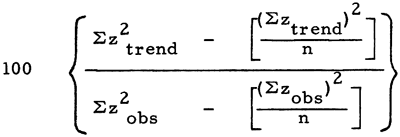
Error measure. Error measure (lines 276 to 281) is defined as the sum of the squared residual values, divided by the number of data points, less one, which may be expressed as follows:

EM = Σ(z_obs - z_trend)² / (n-1)

Error measure is thus a measure of the degree to which the calculated trend approaches the observed data values. A perfectly fitted trend would have an error measure of zero.

Sum of Squares. The sums of squares associated with the linear, quadratic, and abbreviated cubic trend components, and with deviations from these components are calculated (lines 286 to 297, 305). These values may be used to determine confidence levels associated with the components by analysis of variance.

Percent of total sum of squares. Another measure of the degree to which the trend approaches the observed data is the percent of total sum of squares (lines 298 to 304). The percent of total sum of squares may be defined algebraically as:

The percent of total sum of squares may vary from only a few percent to almost 100 percent. A value of 100 percent would indicate a perfect fit of the trend to the observed data.

Calculation of Hypervolumes and Average z Value

The program provides for calculation of four-dimensional hypervolumes within the hypersurfaces between specified limits. If four-dimensional hypervolume is divided by three-dimensional volume, an average value of z is obtained in which the spatial locations of the z data values weight or influence the average. A spatially weighted average calculated in this manner may, in some cases, be more meaningful than the conventional arithmetic mean, particularly where the data values are very irregular and contain extremes. A suggested geological application would be in calculating average porosity values in limestone oil reservoirs, where porosity values obtained by core analysis may be highly erratic.

To explain the principle of this method, analogies have been drawn between calculation of weighted averages where two, three, and four variables are involved (Fig. 14). Consider the problem of obtaining a weighted average of z, where z is a function of x. We may represent the function by a curve (Fig. 14A), and if we wish to calculate the average value of z between limits x1 and x2, we find the area beneath the curve between these limits and then divide by the distance between x1 and x2. Inasmuch as z is expressed as a function of x, the area beneath the curve is obtained by evaluating the integral of the function between the limits x1 and x2. Thus, the average of z is the average height of the curve above the x axis between the limits.

Figure 14--Diagrams and generalized equations showing how spatially weighted average values may be obtained by integration and division where two (A), three (B), and four (C) variables are involved.

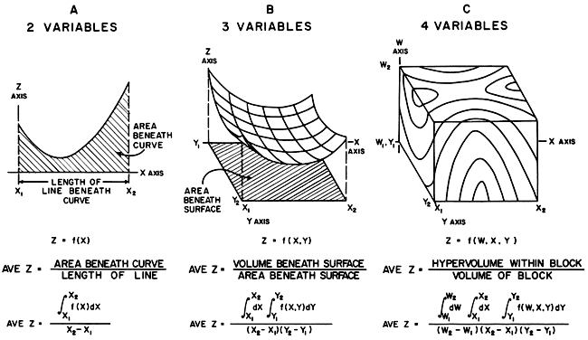
Consider now the problem of calculating a weighted average of z where three variables are involved, and z may be expressed as a function of x and y. Whitten (1962) has discussed the theory of the method in detail. Inasmuch as three variables are involved, a surface (Fig. 14B) rather than a line represents z as a function of x and y. We may think of the weighted average value of z as being the average height of the surface above the x-y plane between the specified limits x₁ to x₂ and y₁ to y₂. To obtain the weighted average we calculate the volume between the surface, the x-y plane, and the four planes specified by x₁, x₂, y₁, and y₂. We then divide this volume by the area in the x-y plane within the limits. The volume is obtained by double integration and evaluation of the integral between the limits.

We may now consider the problem of obtaining a weighted average where four variables are involved, and z may be expressed as a function of w, x, and y and is represented by a hypersurface. The volume within a four-dimensional hypersurface is a four-dimensional hypervolume. When the hypervolume is divided by three-dimensional volume, a weighted average of z is obtained. The principles are the same as with a lesser number of variables. The hypervolume is obtained by evaluation of the triple integral (Fig. 14C) between the three pairs of limits, w₁ to w₂, x₁ to x₂, and y₁ to y₂.

Hypervolume within a first-degree hypersurface. The mathematical steps in obtaining hypervolume within a first-degree hypersurface are outlined below. Hypervolumes within higher-degree hypersurfaces are obtained in the same way, except that the equations have more terms.

The hypervolume within a hypersurface is given by the indefinite triple integral

∫ dw ∫ dx ∫ z dy,

where z is a function of w, x, and y:

z = f(w, x, y)

For a first-degree hypersurface, the function is

z = A + Bw + Cx + Dy

Substituting in this function, we obtain the indefinite triple integral

∫ dw ∫ dx ∫ (A + Bw + Cx + Dy) dy

Integrating with respect to y, we obtain

∫ dw {∫ [Ay + Bwy + Cxy + 1/2 Dy²] dx } dw.

In turn, integrating with respect to x, we obtain

∫ {Axy + Bwxy + 1/2 Cx² y + 1/2 Dxy² } dw

and finally, integrating with respect to w, we obtain

Awxy + 1/2 Bw²xy + 1/2 Cwx²y + 1/2 Dwxy².

We may determine the actual hypervolume by evaluation of the definite integral between specified limits. The general form of the definite triple integral, where z is a function of w, x, and y, may be written

∫w2w1 dw ∫x2x1 dx ∫y2y1 dy

in which the limits represent the values of w, x, and y at the edges of the block in which the hypervolume is to be calculated (Fig. 14C). Thus, the hypervolume is obtained when the equation above is evaluated between these limits by substituting the following values for w, x, and y (lines 355, 358, 361):

w = w₂ - w₁
x = x₂ - x₁
y = y₂ - y₁
w² = w₂² - w₂²
x² = x₂² - x₂²
y² = y₂² - y₂²

The hypervolume between these limits (lines 361 to 365) is given by

Volume = A[(w₂ - w₁)(x₂ - x₁)(y₂ - y₁)]
+ 1/2 B[(w₂² - w₁²)(x₂ - x₁)(y₂ - y₁)]
+ 1/2 C[(w₂ - w₁)(x₂² - x₁²)(y₂ - y₁)]
+ 1/2 D[(w₂ - w₁)(x₂ - x₁)(y₂² - y₁²)]

Hypervolume within second- and third-degree hypersurfaces. The volume within a second-degree hypersurface (lines 355, 356, 358, 359, 361, 362, 367 to 372) is given by the equation:

Volume = A[(w₂ - w₁) (x₂ - x₁) (y₂ - y₁)]
+ 1/2 B[(w₂² - w₁²)(x₂ - x₁)(y₂ - y₁)]
+ 1/2 C[(w₂ - w₁)(x₂² - x₁²)(y₂ - y₁)]
+ 1/2 D[(w₂ - w₁)(x₂ - x₁)(y₂² - y₁²)]
+ 1/3 E[(w₂ - w₁)(x₂³ - x₁³)(y₂ - y₁)]
+ 1/3 F[(w₂ - w₁)(x₂ - x₁)(y₂³ - y₁³)]
+ 1/3 G[(w₂³ - w₁³)(x₂ - x₁)(y₂ - y₁)]
+ 1/4 H[(w₂ - w₁)(x₂² - x₁²)(y₂² - y₁²)]
+ 1/4 I[(w₂² - w₁²)(x₂² - x₁²)(y₂ - y₁)]
+ 1/4 J[(w₂² - w₁²)(x₂ - x₁)(y₂² - y₁²)]

The expression for hypervolume within a third-degree hypersurface (lines 354 to 363, 374 to 379) is not given here. Cubic cross-product terms have been omitted in the program for the third-degree hypersurface, cutting down substantially on the number of arithmetic operations in evaluating the expression.

Contouring of Intersection of Hypersurface with a Plane

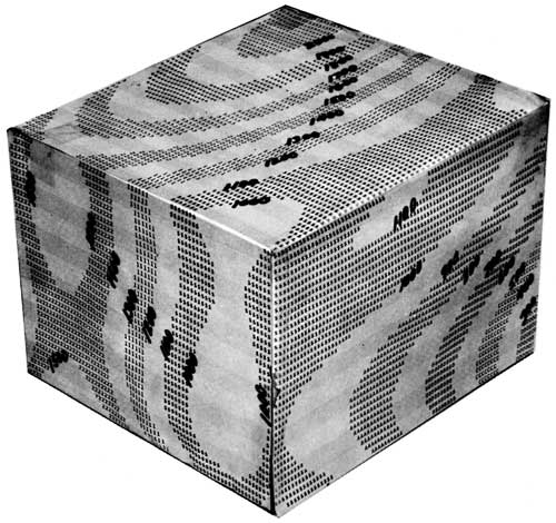
A hypersurface can be visualized by passing planes through it and contouring the values of the hypersurface where they intersect the planes. In this program, planes are contoured one at a time (Appendix C, Part 2) and may be pasted together later to form a rectangular block (Fig. 15).

Figure 15--Hypersurface block constructed by pasting together surfaces on which contour bands have been printed by computer's printing machine. Numbers denoting values of edges of bands were put on by hand.

Contouring (lines 426 to 689) is accomplished by holding constant the coordinate value (w, x, or y) that specifies the plane, progressively varying the other two coordinates values, and solving for z with the equation describing the hypersurface. Values assigned to the two coordinates are progressively changed according to the spacing in columns and rows of the printed characters of the computer's printing machine (an IBM 1403 high-speed printer has been used in the examples shown).

After the value of z has been determined at a particular point on the plane on which the contours are being drawn, either a blank space or a certain character, which may be a number, letter, or other character (Table 7) is printed. The character printed depends on the value of z at that point, the reference contour value, and the contour interval value. The printed characters have been arranged so that there is little likelihood of ambiguity. The steps in calculating the values of contour lines are as follows:

1. Determine the number of contour intervals represented by the band of characters or blanks by referring to Table 7.
2. Multiply this number by the contour interval.
3. Add algebraically to the reference contour value.

For example, if the contour value is 100, and the contour interval is 10, then the contour value represented by the algebraically lower edge of the band printed with B's is 60. The reference contour value is marked by the edge of the band of $'s which faces the band of A's.

Plotting of Original Data and of Residual Values

In this program, all plotting of data points is done automatically. It is possible to do this because the location of each data point is specified by the coordinate values w, x, and y. Plotting of points on an ordinary map is usually no problem because the location of any point can be specified by two coordinate values, x and y. But, plotting of points in three-dimensional space poses a problem. In this program (lines 690 to 750) points are plotted by dividing the three-dimensional block (Fig. 11A) into a series of horizontal slices (Appendix C, Part 3), each slice being of specified constant thickness. Data points within a slice are projected onto a plane and plotted as points on an ordinary map. The number of maps plotted equals the number of slices. This approach does not completely avoid the difficulty of plotting points in three-dimensional space because differences in elevation of points within a slice are ignored. However, it is a practical approach to a problem that has no simple solution.

Table 7--List of characters that correspond with contour intervals of printed contour maps. Empty places in column indicate that no character is printed.

In the program the values must be sorted before they are plotted. First, the values are sorted according to the w-coordinate values, which in a subsurface geological application would be according to depth. The values are then assigned to appropriate slices, sorted according to y-coordinate values, and finally sorted according to x-coordinate values. The data points within each slice are plotted at the approximate locations specified by their x- and y-coordinate values. The number printed for each point is located so that its right edge generally corresponds with the actual map location of the data point. Spaces between points are left blank. Of course, small errors are introduced because the numbers are confined to the printer's columns and rows, which are spaced 1/10 and 1/6 of an inch apart, respectively. Additional errors may be introduced where the points are very close together so that the printed numbers tend to overlap. Because all the characters in each line or row are printed simultaneously, printed characters cannot overlap. To avoid this mechanical problem, the location of each printed point is shifted to the right where it would tend to overlap the number representing the data point immediately to the left. At least one blank space is left between numbers, except where a minus sign is present. All numbers are truncated to integers to save space in printing.

As noted previously, thickness of the slices and the w-coordinate values of the upper surfaces of the uppermost and the lowermost slice must be specified in the input data. In the program, the original data values are plotted first, followed successively by the first-, second-, and third-degree residual values.

Appendix B

Listing of Computer Program for Fitting Hypersurfaces

Each line has been arbitrarily numbered for identification at left edge of the line. In actual practice identification numbers are confined to columns 73 to 80 on the punch cards, and 2 is necessary in column 1.

[Note on web version: Code was proofread from original printed text, which was not particularly clear. There are bound to be errors.]

  1   COMMENT PROGRAM 15, FITS 4TH DIMENSIONAL 1ST, 2ND, AND 3RD DEGREE
  2   VOLUMES BY LEAST SQUARES TO IRREGULARLY SPACED DATA POINTS, VOLUMES
  3   CALCULATED BY TRIPLE INTEGRATION AND HORIZONTAL SURFACES ARE CONTOURED.
  4   J.W. HARBAUGH, GEOLOGY DEPT., STANFORD $
  5   INTEGER  XP(), I, J, K, L, OP, N, VERT, HOR, CV(), EL, M, W $
  6   INTEGER ARMIN, ARPLS, YDIM, WDIM, LY, LX, DIGITS, N2 $
  7   INTEGER PLTAR, PRINT, IY, IX, C= TEMP, LINE $
  8   ARRAY PRINT(3,50), IY(950), IX(950), DIGITS(50) $
  9   ARRAY   PLTAR(12)= ('Z VALU','ES ORI','G DATA','1STDEG',
 10           'REE RE','SIDUAL','2NDDEG','REE RE','SIDUAL','3RDDEG',
 11           'REE RE','SIDUAL') $
 12   INTEGER 12 $ ARRAY 12(950)$
 13   ARRAY ARMIN(40) = (' ','A',' ','B',' ','C',' ','D',' ','E',' ','F','
 14      '','G',' ','H',' ','I',' ','J',' ','K',' ','L',' ','M',' ','N','
 15      '','O',' ','P',' ','Q',' ','R',' ','S',' ','T',') $
 16   ARRAY ARPLS(40) = ('$',' ','1',' ','2',' ','3',' ','4',' ','5',' ',
 17      '6',' ','7',' ','8',' ','9',' ','0',' ','$',' ','*',' ','-',' ',
 18      '.',' ','+',' ','=',' ','W',' ','X',' ','Y',' ') $
 19   ARRAY X(950,10),T(13,13),R(13), XP(950,4), T4(6,6), T10(12,12),
 20   T13(15,I5), R4(4), R10(10), R(13), XP(950,4), T4(6,6), T10(12,12),
 21   CV(132), LEV(20), LEX(20), LAY(20) $
 22   FORMAT FORM($K$(B$PRINT(3,I)$,I$ DIGITS(I)$),W)$
 23   OUTPUT PLOT(PLTAR((1,5(C-1))-3,5), PLTAR((1,5(C-1))-2,5),
 24   PLTAR(1,5(C-2))) $
 25   FORMAT PLFT(3A6,W,W) $
 26   FORMAT RESLEV( *LOWER LEVEL OF SLICE = *,X8,2,*   UPPER LEVEL *,
 27      *OF SLICE =   *, X8,2, W,W)$
 28   OUTPUT RESOUT      (FWSTEP, FW)$
 29   START,,
 30   INPUT ALPH(Al,A2,A3,A4,A5,A6,A7,A8,A9,A10,A11,A12)   $
 31   READ ($$ ALPH) $
 32   INPUT PREF( OP, N, YDIM, HOR, XR, XL, YB, YT, WB, WT, RF, CON,
 33   WDIM, PUNCHOP, RESIDOP)$
 34   READ ($$ PREF)$
 35   INPUT ELVS(EL,FOR I = (1,1,EL) $ LEV(I))$ READ ($$ ELVS)$
 36   INPUT LXVS(LX,FOR I = (1,1,LX) $ LEX(I))$ READ ($$ LXVS)$
 37   INPUT LYVS(LY,FOR I = (1,1,LY) $ LAY(I))$ READ ($$ LYVS)$
 38   IF RESIDOP EQL 1 $(INPUT RPLOTCON(LOW,STEP,HIGH)$ READ($$RPLOTCON))$
 39   YDAM = YDIM $ HAR = HOR $
 40   IF OP EQL 2222 $
 41      BEGIN
 42         INPUT DATI(FOR I =(1,1,N) $ FOR J =(1,1,4) $ XP(I,J))$
 43         READ ($$ DATI) $
 44         FOR I =(1,1,N) $ FOR J =(1,1,4) $ X(I,J) = XP(I,J) S
 45      END $
 46   IF OP EQL 4444 $
 47      BEGIN
 48         INPUT DATD(FOR I =(1,1,N) $ FOR J =(1,1,4) $ X(I,J)) $
 49         READ ($$ DATD) $
 50      END $
 51   FOR K = (1,1,13) $ FOR L = (1,1,13) $ T(K,L) = 0.0 $
 52   FOR K = (1,1,13) $ R(K) = 0.0 $
 53   COMMENT CALCULATE VALUES FOR 13 X 13 T MATRIX ELEMENTS, EXCEPT FOR
 54   THOSE VALUES THAT ARE DUPLICATES OF OTHERS, WHICH WILL BE ASSIGNED $
 55   FOR I = (1,1,N) $
 56   BEGIN
 57   T(1,2)  = T(1,2) + X(I,1) $
 58   T(1,3)  = T(1,3) + X(I,2) $
 59   T(1,4)  = T(1,4) + X(I,3) $
 60   T(1,5)  = T(1,5) + (X(I,2).X(I,2)) $
 61   T(1,6)  = T(1,6) + (X(I,1).X(I,3)) $
 62   T(1,7)  = T(1,7) + (X(I,2).X(I,3)) $
 63   T(1,8)  = T(1,8) + (X(I,1).X(I,2)) $
 64   T(1,9)  = T(1,9) + (X(I,1).X(I,1)) $
 65   T(1,10) = T(1,10) + (X(I,3).X(I,3)) $
 66   T(2,5)  = T(2,5) + (X(I,1).(X(I,2).X(I,2))) $
 67   T(2,6)  = T(2,6) + (X(I,1).(X(I,1).X(I,3))) $
 68   T(2,7)  = T(2,7) + (X(I,1).(X(I,2).X(I,3))) $
 69   T(2,8)  = T(2,8) + (X(I,1).(X(I,1).X(I,2))) $
 70   T(2,9)  = T(2,9) + (X(I,1).(X(I,1).X(I,1))) $
 71   T(2,10) = T(2,10) + (X(I,1).(X(I,3).X(I,3))) $
 72   T(3,5)  = T(3,5) + (X(I,2).(X(I,2).X(I,2)))   $
 73   T(3,7)  = T(3,7) + (X(I,2).(X(I,2).X(I,3))) $
 74   T(3,10) = T(3,10) + (X(I,2).(X(I,3).X(I,3))) $
 75   T(4,10) = T(4,10) + (X(I,3).(X(I,3).X(I,3)))$
 76   T(5,5)  = T(5,5) + ((X(I,2).X(I,2)).(X(I,2).X(I,2))) $
 77   T(5,6)  = T(5,6) + ((X(I,1).X(I,2)).(X(I,2).X(I,3))) $
 78   T(5,7)  = T(5,7) + ((X(I,2).X(I,2)).(X(I,2).X(I,3))) $
 79   T(5,8)  = T(5,8) + ((X(I,1).X(I,2)).(X(I,2).X(I,2))) $
 80   T(5,9)  = T(5,9) + ((X(I,1).X(I,1)).(X(I,2).X(I,2))) $
 81   T(5,10) = T(5,10) + ((X(I,2).X(I,2)).(X(I,3).X(I,3))) $
 82   T(6,6)  = T(6,6) + ((X(I,1).X(I,1)).(X(I,3).X(I,3))) $
 83   T(6,7)  = T(6,7) + ((X(I,1).X(I,2)).(X(I,3).X(I,3))) $
 84   T(6,8)  = T(6,8) + ((X(I,1).X(I,1)).(X(I,2).X(I,3))) $
 85   T(6,10) = T(6,10) + ((X(I,1).X(I,3)).(X(I,3).X(I,3))) $
 86   T(7,10) = T(7,10) + ((X(I,2).X(I,3)).(X(I,3).X(I,3))) $
 87   T(8,9)  = T(8,9) + ((X(I,1).X(I,1)).(X(I,1).X(I,2))) $
 88   T(6,9)  = T(6,9) + ((X(I,1).X(Il,1)).(X(I,1).X(I,3))) $
 89   T(9,9)  = T(9,9) + ((X(I,1).X(I,1)).(X(I,1).X(I,1))) $
 90   T(9,10) = T(9,10) + ((X(I,1).X(I,1)).(X(I,3).X(I,3))) $
 91   T(10,l0) = T(10,10) + ((X(I,3).X(I,3)).(X(I,3).X(I,3))) $
 92   T( 5,11) = T( 5,11) + ((X(I,2).X(I,2)).(X(I,2).X(I,2).X(I,2)))) $
 93   T( 5,12) = T( 5,12) + ((X(I,1).X(I,1)).(X(I,1).(X(I,2).X(I,2)))) $
 94   T( 5,13) = T( 5,13) + ((X(I,2).X(I,2)).(X(I,3).(X(I,3).X(I,3)))) $
 95   T( 6,11) = T( 6,11) + ((X(I,1).X(I,2)).(X(I,2).(X(I,2).X(I,3)))) $
 96   T( 6,12) = T( 6,12) + ((X(I,1).X(I,1)).(X(I,1).(X(I,1).X(I,3)))) $
 97   T( 6,13) = T( 6,13) + ((X(I,1).X(I,1)).(X(I,3).(X(I,3).X(I,3)))) $
 98   T( 7,11) = T( 7,11) + ((X(I,2).X(I,2)).(X(I,2).(X(I,2).X(I,3)))) $
 99   T( 7,12) = T( 7,12) + ((X(I,1).X(I,1)).(X(I,1).(X(I,2).X(I,3)))) $
100   T( 7,13) = T( 7,13) + ((X(I,2).X(I,3)).(X(I,3).(X(I,3).X(I,3)))) $
101   T( 8,11) = T( 8,11) + ((X(I,1).X(I,2)).(X(I,2).(X(I,2).X(I,2)))) $
102   T( 8,12) = T( 8,12) + ((X(I,1).X(I,1)).(X(I,1).(X(I,1).X(I,2)))) $
103   T( 8,13) = T( 8,13) + ((X(I,1).X(I,2)).(X(I,3).(X(I,3).X(I,3)))) $
104   T( 9,11) = T( 9,11) + ((X(I,1).X(I,1)).(X(I,2).(X(I,2).X(I,2)))) $
105   T( 9,12) = T( 9,12) + ((X(I,1).X(I,1)).(X(I,1).(X(I,1).X(I,1)))) $
106   T( 9,13) = T( 9,13) + ((X(I,1).X(I,1)).(X(I,3).(X(I,3).X(I,3)))) $
107   T(10,11) = T(10,11) + ((X(I,2).X(I,2)).(X(I,2).(X(I,3).X(I,3)))) $
108   T(10,12) = T(10,12) + ((X(I,1).X(I,1)).(X(I,1).(X(I,3).X(I,3)))) $
109   T(10,13) = T(10,13) + ((X(I,3).X(I,3)).(X(I,3).(X(I,3).X(I,3)))) $
110   T(11,11) = T(11,11) + ((X(I,2).(X(I,2).X(I,2))).(X(I,2).(X(I,2).X(I,2)))) $
1ll   T(11,12) = T(11,12) + ((X(I,1).(X(I,1).X(I,1))).(X(I,2).(X(I,2).X(I,2)))) $
112   T(11,13) = T(11,13) + ((X(I,2).(X(I,2).X(I,2))).(X(I,3).(X(I,3).X(I,3)))) $
113   T(12,12) = T(12,12) + ((X(I,1).(X(I,1).X(I,1))).(X(I,1).(X(I,1).X(I,1)))) $
114   T(12,13) = T(12,13) + ((X(I,1).(X(I,1).X(I,1))).(X(I,3).(X(I,3).X(I,3)))) $
115   T(13,13) = T(13,13) + ((X(I,3).(X(I,3).X(I,3))).(X(I,3).(X(I,3).X(I,3)))) $
116   R(1 ) = R(1 ) + X(I,4) $
117   R(2 ) = R(2 ) + (X(I,4).X(I,1)) $
118   R(3 ) = R(3 ) + (X(I,4).X(I,2)) $
119   R(4 ) = R(4 ) + (X(I,4).X(I,3)) $
120   R(5 ) = R(5 ) + (X(I,4).(X(I,2).X(I,2))) $
121   R(6 ) = R(6 ) + (X(I,4).(X(I,1).X(I,3))) $
122   R(7 ) = R(7 ) + (X(I,4).(X(I,2).X(I,3))) $
123   R(8 ) = R(8 ) + (X(I,4).(X(I,1).X(I,2))) $
124   R(9 ) = R(9 ) + (X(I,4).(X(I,1).X(I,1))) $
125   R(10) = R(10) + (X(I,4).(X(I,3).X(I,3))) $
126   R(11) = R(11) + ((X(I,4).X(I,2)).(X(I,2).X(I,2))) $
127   R(12) = R(12) + ((X(I,4).X(I,1)).(X(I,1).X(I,1))) $
128   R(13) = R(13) + ((X(I,4).X(I,3)).(X(I,3).X(I,3))) $
129   END $
130   T(1,1) = N S
131   T(2,1) = T(1,2) $ T(1,11) = T(3,5) $
132   T(2,2) = T(1,9) $ T(1,12) = T(2,9) $
133   T(2,3) = T(1,8) $ T(1,13) = T(4,10) $
134   T(2,4) = T(1,6) $ T(2,11) = T(5,8) $
135   T(3,1) = T(1,3) $ T(2,12) = T(9,9) $
136   T(3,2) = T(1,8) $ T(2,13) = T(6,10) $
137   T(3,3) = T(1,5) $ T(3,l1) = T(5,5) $
138   T(3,4) = T(1,7) $ T(3,12) = T(8,9) $
139   T(3,6) = T(2,7) $ T(3,13) = T(1,97) $
140   T(3,8) = T(2,5) $ T(4,l1) = T(5,7) $
141   T(3,9) = T(2,8) $ T(4,12) = T(6,9) $
142   T(4,1) = T(1,4) $ T(4,13) = T(10,10) $
143   T(4,2) = T(1,6) $ T(11,1) = T(1,11) $
144   T(4,3) = T(1,7) $ T(11,2) = T(2,11) $
145   T(4,4) = T(1,10) $ T(11,3) = T(3,11) $
146   T(4,5) = T(3,7) $ T(11,4) = T(4,11) $
147   T(4,6) = T(2,10) $ T(11,5) = T(5,11) $
148   T(4,7) = T(3,10) $ T(11,6) = T(6,11) $
149   T(4,8) = T(2,7) $ T(11,7) = T(7,11) $
150   T(4,9) = T(2,6) $ T(11,8) = T(8,11) $
151   T(5,1) = T(1,5) $ T(11,9) = T(9,11) $
152   T(5,2) = T(2,5) $ T(11,10) = T(10,11) $
153   T(5,3) = T(3,5) $ T(12,1) = T(1,12) $
154   T(5,4) = T(3,7) $ T(12,2) = T(2,12) $
155   T(6,1) = T(1,6) $ T(12,3) = T(3,12) $
156   T(6,2) = T(2,6) $ T(12,4) = T(4,12) $
157   T(6,3) = T(2,7) $ T(12,5) = T(5,12) $
158   T(6,4) = T(2,10) $ T(12,6) = T(6,12) $
159   T(6,5) = T(5,6) $ T(12,7) = T(7,12) $
260   T(7,1) = T(1,7) $ T(12,8) = T(8,12) $
161   T(7,2) = T(2,7) $ T(12,9) = T(9,12) $
162   T(7,3) = T(3,7) $ T(12,10) = T(10,12) $
163   T(7,4) = T(3,10) $ T(13,1) = T(1,13) $
164   T(7,5) = T(5,7) $ T(13,2) = T(2,13) $
165   T(7,6) = T(6,7) $ T(13,3) = T(7,10) $
166   T(7,7) = T(5,10) $ T(13,4) = T(4,13) $
167   T(7,8) = T(5,6) $ T(13,5) = T(5,13) $
168   T(7,9) = T(6,8) $ T(13,6) = T(6,13) $
169   T(8,1) = T(1,8) $ T(13,7) = T(7,13) $
170   T(8,2) = T(2,8) $ T(13,8) = T(8,13) $
171   T(8,3) = T(2,5) $ T(13,9 = T(9,13) $
172   T(8,4) = T(2,7) $ T(13,10 = T(10,23) $
173   T(8,5) = T(5,8) $ T(12,11) = T(11,12) $
174   T(8,6) = T(6,8) $ T(13,11) = T(11,13) $
175   T(8,7) = T(5,6) $ T(13,12) = T(12,13) $
176   T(8,8) = T(5,9) $ T(3,13) = T(7,10) $
177   T(8,10) = T(6,7) $
178   T(9,1) = T(1,9) $
179   T(9,2) = T(2,9) $
180   T(9,3) = T(2,8) $
181   T(9,4) = T(2,6) $
182   T(9,5) = T(5,9) $
183   T(9,6) = T(6,9) $
184   T(9,7) = T(6,8) $
185   T(9,8) = T(8,9) $
186   T(10,1) = T(1,10) $
187   T(10,2) = T(2,10) $
188   T(10,3) = T(3,10) $
189   T(10,4) = T(4,10) $
190   T(10,5) = T(5,10) $
191   T(10,6) = T(6,l0) $
192   T(10,7) = T(7,10) $
193   T(10,8) = T(6,7) $
194   T(10,9) = T(9,10) $
195   FOR I = (1,1,4)$ FOR J = (1,1,4) $T4(I,J) = T(I,J) $
196   FOR I = (1,1,13)$ FOR J = (1,1,13) $T13(I,J) = T(I,J) $
197   FOR I = (1,1,10)$ FOR J = (1,1,10) $T10(I,J) = T(I,J) $
198   COMMENT ASSIGN 4, 10, AND 13 PORTIONS OF COLUMN VECTOR R TO NEW VECTORS$
199   FOR I = (1,1,4) $ R4(I) = R(I) $
200   FOR I = (1,1,13) $ R13(I) = R(I) $
201   FOR I = (1,1,10) $ R10(I) = R(I) $
202   COMMENT SOLVE LINEAR MATRIX EQUATIONS OF GENERAL FORM TS = R $
203   EXTERNAL PROCEDURE INPROD() $
204   PROCEDURE SOLV(N$A(,),B(),Y()$SINGULAR) $
205   BEGIN
206   COMMENT THIS IS THE METHOD OF CROUT,WITH INTERCHANGES,
207      TO SOLVE AY=B FOR Y,GIVEN A AND B. $
208      COMMENT EXTERNAL PROCEDURE INPROD IS CALLED BY SOLV,
209      SO INPROD MUST BE AVAILABLE WHEN SOLV IS CALLED. $
210   COMMENT SINGULAR IS THE LABEL OF THE STATEMENT TO WHICH
211      SOLV() EXITS IF A() 1S SINGULAR $
222   COMMENT REAL A(,)B(),Y() $
213   INTEGER I,IMAX,J,K,N $
214      FOR K=(1,1,N) $
215      BEGIN
216         TEMP = 0 $
217         FOR I = (K,1,N) $
218         BEGIN
219            XX = A(I,K) - INPROD(1,1,K-1,A(I,),A(,K)) $
220            A(I,K) = XX $
221            IF ASS(XX) GTR TEMP
222            BEGIN
223               TEMP = ABS(XXH $
224               IMAX = 1
225            END
226        END $
227        IF TEMP EQL 0.0 $
228        GO SINGULAR $
229      COMMENT WE HAVE FOUND THAT A(IMAX,K) IS THE LARGEST PIVOT IN COL K.
230        NOW WE INTERCHANGE ROWS K AND IMAX $
231      IF IMAX NEQ K $
232      BEGIN
233         FOR J = (1,1,N)$
234         BEGIN
235            TEMP = A(K,J)$ A(K,J) = A(IMAX,J)$ A(IMAX,J) = TEMP
236         END $
237         TEMP = B(K)$B(K) = B(IMAX)$B(IMAX) = TEMP
238      END $
239      COMMENT NOW FOR THE ELIMINATION $
240      DENOM = A(K,K) $
241      FOR I =(K+1,1,N) $
242      A(I,K) = A(I,K)/DENOM $
243      FOR J = (K+1,1,N) $
244         A(K,J) = A(K,J) - INPROD(1,1,K-1,A(K,),A(J)) $
245      B(K) = B(K) - INPROD(1,1,K-1,A(K,),B())
246    END $
247     FOR I = (1,1,N)$ Y(I) = A(I,I) $
248    COMMENT NOW FOR THE BACK SUBSTITUTION $
249    FOR K = (N,-1,1) $
250      Y(K) = (B(K) - INPROD(K+1,K+1,N-K,A(K,),Y()))/A(K,K) $
251     RETURN
252   END SOLV() $
253   SOLV( 4$ T4(,), R4(), Q() $ MAT6) $
254   MAT6..
255   SOLV(10$T10(,),R10(), S() $ MAT10) $
256   MAT10..
257   SOLV(13$T13(,)R13(), F() $ START) $
258   COMMENT SUBSTITUTE W,X AND Y VALUES IN EQUATIONS OF FITTED SURFACES $
259   FOR I = (1,1,N) $
260   BEGIN
261   X(I,5) = Q(1) + (Q(2).X(I,1)) + (Q(3).X(I,2)) + (Q(4).X(I,3)) $
262   X(I,6) = X(I,4) - X(I,5) $
263   X(I,7) = S(1) + (S(2).X(I,1)) + (S(3).X(I,2)) + (S(4).X(I,3)) +
264      (S(5).(X(I,2).X(I,2))) + (S(6).(X(I,1).X(I,3))) +
265      (S(7).(X(I,2).X(I,3))) + (S(8).(X(I,1).X(I,2))) +
266      (S(9).(X(I,1).X(I,1))) + (S(10).(X(I,3).X(I,3))) +
267   X(I,8) = X(I,4) - X(I,7) $
268   X(I,9) = F(1) + (F(2).X(I,1)) + (F(3).X(I,2)) + (F(4).X(I,3)) +
269      (F(5).(X(I,2).X(I,2))) + (F(6).(X(I,1).X(I,3))) +
270      (F(7).(X(I,2).X(I,3))) + (F(B).(X(I,1).X(I,2))) +
271      (F(9).(X(I,1).X(I,1))) + (F(10).(X(I,3).X(I,3))) +
272      ((F(11).X(I,2)).(X(I,2).X(I,2))) + ((F(12).X(I,1)).(X(I,1).X(I,1)))+
273      ((F(13).X(I,3)).(X(I,3).X(I,3))) $
274   X(I,10) = X(I,4) - X(I,9) $
275   END   $
276   EM1 = EM2 = EM3 = 0.0 $
277   FOR I = (1,1,N) $
278      BEGIN
279         EM1 = EM1 +(X(I,6).X(I,6)) $
280         EM2 = EM2 +(X(I,8).X(I,8)) $
281         EM3 = EM3 +(X(I,10).X(I,10)) $
282      END $
283      E1 = EM1/(N-1) $
284      E2 = EM2/(N-1) S
285      E3 = EM3/(N-1) $
286   SMLN = LNSQ = SMQD = ODSQ = SMCB = CBSQ = SMZ = ZSQ = 0.0 $
287   FOR I = (1,1,N) $
288      BEGIN
289         SMLN = SMLN + X(I,5) S
290         LNSQ = LNSO + (X(I,5).X(I,5)) $
291         SMQD = SMQD + X(I,7) $
292         QDSQ = QDSQ + (X(I,7).X(I,7)) $
293         SMCB = SMCB + X(I,9) $
294         CBSQ = CBSO + (X(I,9).X(I,9)) $
295         SMZ = SMZ + X(I,4) $
296         ZSQ = ZSQ + (X(I,4).X(I,4)) $
297      END $
298   ZOR = ZSQ - ((SMZ,SMZ)/(N-1)) $
299   PTS1 = 100.0((LNSQ-((SMLN.SMLN)/(N-1)))/ZOR) $
300   PTS2 = 100.0((QDSQ-((SMQD.SMQD)/(N-1)))/ZOR) $
301   PTS3 = 100.0((CBSQ-((SMCB.SMCB)/(N-1)))/ZOR) $
302   IF PTS1 LSS 0.0 $ PTS1 = 100.0 + PTS1 $
303   IF PTS2 LSS 0.0 $ PTS2 = 100.0 + PTS2 $
304   IF PTS3 LSS 0.0 $ PTS3 = 100.0 + PTS3 $
305   QDON = QDSQ - LNSQ $ CBON = CB2Q - QDSQ $
306   OUTPUT ERMA(E1 ,E2 ,E3 ,PTS1,PTS2,PTS3) $
307   FORMAT FMTR(*ERROR MEASURE LINEAR TREND SURFACE = *,X31.2,W,W,
308               *ERROR MEASURE QUADRATIC TREND SURFACE = *,X28.2,W,W,
309               *ERROR MEASURE CUBIC TREND SURFACE = *,X32.2,W,W,
310               *PERCENT TOTAL SUM SQUARES LINEAR SURFACE = *,X25.2,W,W,
311               *PERCENT TOTAL SUM SQUARES QUADRATIC 5URFACE = *,X22.2,W,W,
312               *PERCENT TOTAL SUM SQUARES CUBIC SURFACE = *,X26.2,W,W) $
313   OUTPUT VAR(LNSQ, EM1, QDSQ, QDON, EM2, CBSQ, EM3, CBON   ) $
314   FORMAT FVAR(*SUM OF SQUARES DUE LINEAR COMPONENT = *,X30,2,W4,W,
315               *SUM OF SQUARED DEVIATIONS FROM LINEAR = *,X28.2,W,W,
316               *SUM OF SQUARES DUE LINEAR + QUADRATIC COMPONENT = *,Xl8.2,
317           W,W,*SUM OF SQUARES DUE TO QUADRATIC ALONE = *,X28.2,W,W,
318               *SUM OF SQUARED DEVIATIONS FROM LINEAR + QUADRATIC = *,
319               X16.2,W,W,
320               *SUM OF SQUARES DUE LINEAR+QUADRATIC+CUBIC = *,X24,2,W,W,
321               *SUM OF SQUARED DEVIATIONS FROM LINEAR+QUADRATIC+CUBIC = *,
322               X12.2,W,W,
323               *SUM OF SQUARES DUE CUBIC ALONE = *,X35,2,W, W)$
324   AZM = R(1)/N $
325   OUTPUT ALPHA(A1,A2,A3,A4,A5,A6,A7,A8,A9,A10,A11,A12) $
326   OUTPUT ODS1(FOR I = (1,1,N) $ FOR J = (1,1,10) $ X(I,J)) $
327   FORMAT FMTA(12A6,W3,W) $
328   OUTPUT C03(FOR J = (1,1,4) $ Q(J)),
329          C06(FOR J = (1,1,10) $ S(J)),
330          C10(FOR J = (1,1,13) $ F(J)) $
331   FORMAT CF3(W,*EQUATION COEFFICIENTS *,W,*LINEAR, Z = *,X12.5,*+*,
332         X12.7,*W + *,X12.7,*X + *,X12.7,*Y*,W,W),
333         CF6(*LIN + QUAD, Z = *,X12.5,* + *,X12.7,*W + *,X12.7,*X + *,X12.7,
334         *Y + *,X12.8,*X2 + *,X12.8,*WY + *,X12.8,*XY*,W,W,B10,
335         * + *,X12.8,*WX + *,X12.8,*W2 + *,X12.8,*Y2*,W,W),
336         CF10(*LIN + QUAD + CUB, Z = *,X12.5,* + *,X12.7,*W + *,X12.7,*X + *,
337         X12.7,*Y + *,X12.8,*X2 + *,X12.8,*WY*,W,W,B10,* + *,X12.8,*XY + *,
338         X12.8,*WX + *,X12.8,*W2 + *,X12.8,*Y2 + *,X12.8,*X3 + *,X12.8,
339         *W3 + *,X12.8,*Y3*,W,W) $
340   FORMAT HED(W,*WCOORD *,
341          *XCOORD YCOORD Z-VALUE 1ST-TRD 1ST-RSD 2ND-TRD 2ND-RSD*,
342          * 3RD-TRD 3RD-RSD*,W,W) $
343   FORMAT FMT1(*5*, X7.1, 9X8.l, W) $
344   FORMAT FMT2(*5*, X7.1, 9X8.1, C) $
345   FORMAT FMTAP(*5$*, 12A6, *$*, W) $
346   WRITE ($$ ALPHA, FMTA) $
347   FORMAT JIM(*13 X 13 (X,Y) MATRIX VALUES *,W,W) $ WRITE ($$ JIM) $
348   OUTPUT TRAY(FOR I = (1,1,13)$ FOR J = (1,1,13) $ T(I,J)) $
349   FORMAT FTRA(W,13F10.3,W) $
350   WRITE ($$ TRAY,FTRA) $
351   FORMAT JOE(W,*1 X 13 COLUMN VECTOR VALUES*,W,W) $ WRITE ($$ JOE) $
352   OUTPUT RAR(FOR I = (1,1,13) $ R(1)) $ WRITE ($$ RAR, FTRA) $
353   WRITE ($$ C03, CF3) $ WRITE ($$ C06, CF6)$ WRITE ($$ C10, CF10) $
354   WRITE (S$ ERMA, FMTR) $ WRITE '$$ VAR, FVAR) $
355   WD1 = WB - WBT $ WD2 = (WB.WB) - (WT.WT) $
356   WD3 = (WB.(WB.WB)) - (WT.(WT.WT)) $
357   WD4 = ((WB.WB).(WB.WB)) - ((WT.WT).(WT.WT)) $
358   XD1 = XR - XL $ XD2 = (XR.XR) - (XL.XL) $
359   XD3 = (XR.(XR.XR)) - (XL.(XL.XL)) $
360   XD4 = ((XR.XR).(XR.XR)) - ((XL.XL).(XL.XL)) $
361   YD1 = YB - YT $ YD2 = (YB.YB) - (YT.YT) $
362   YD3 = (YB.(YB.YB)) - (YT.(YT.YT)) $
363   YD4 = ((YB.YB).(YB.YB)) - ((YT.YT).(YT.YT)) $
364   AR = WD1.(XD1.YD1) $
365   VLN = ((Q(1).WD1).(XD1.YD1)) + (((0.5).Q(2)).(WD2.(XD1.YD1)))
366      +(((0.5).Q(3)).(WD1.(XD2.YD1))) + (((0.5).Q(4)).(WDI.(XD1.YD2)))$
367   VQD = ((S(1).WD1).(XD1.YD1)) + (((0.5).S(2)).(WD2.(XD1.YD1)))
368      +(((0.5).S(3)).(WD1.(XD2.YD1))) + (((0.5). S(4)).(WD1.(XD1.YD2)))
369      +(((O.3333).S(5)).(WD1.(XD3.YD1))) + (((0.25).S(6)).(WD2.(XD1.YD2)))
370      +(((0.25).S(7)).(WD1.(XD2.YD2))) + (((0.25).S(8)).(WD2.(XD2.YD1)))
371      +(((0.3333).S(9)).(WD3.(XD1.YD1)))
372      +(((0.3333).S(10)).(WD1.(XDl.YD3))) $
373   VCB = ((F(1).WD1).(XD1.YD1)) + (((0.5).F(2)).(WD2.(XD1.YD1))) +
374   (((0.5).F(3)).(WD1.(XD2.YD1))) + (((0.5).F(4)).(WD1.(XD1.YD2))) +
375   (((0.3333).F(5)).(WD1.(XD3.YD1))) + (((0.25).F(6)).(WD2.(XD1.YD2))) +
376   (((0.25).F(7)).(WD1.(XD2.YD2))) + (((0.25).F(8)).(WD2.(XD2.YD1))) +
377   (((0.3333).F(9)).(WD3.(XD1.YD1)))+ (((0.3333).F(10)).(WD1.(XD1.YD3))) +
378   (((0.25).F(11)).(WD1.(XD4.YD1))) + (((0.25).F(12)).(WD4.(XD1.YD1))) +
379   (((0.25).F(13)).(WD1.(XD1.YD4))) $
380   AZ1 = VLN/AR $ AZ2 = VQD/AR $
381   AZ3 = VCB/AR $
382   OUTPUT VOL(VLN, VQD, VCB, AZM, AZ1, AZ2, AZ3, AR) $
383   FORMAT FMVL(W,*VOLUME WITHIN LINEAR SURFACE = *,B8,X12.2,W,W,
384                 *VOLUME WITHIN LIN + QUAD SURFACE = *,B6,X12.2,W,W,
385                 *VOLUME WITHIN LIN + QUAD + CUB SURFACE = *,B2,X12.2,W,W,
386                 *ARITH. MEAN Z, = SUM OF Z VALUES/N = *,X11.2,W,W,
387                 *AVERAGE Z VALUE, LINEAR SURFACE = *,B6,X12.2,W,W,
388                 *AVERAGE Z VALUE, LIN + QUAD SURFACE = *,B4,X12.2,W,W,
389                 *AVERAGE Z VALUE, LIN + QUAD + CUB SURFACE = *,X12.2,W,W,
390                 *VOL OF BLOCK IN CUBED UNITS*,B11,X12.2,W,W) $
391   WRITE ($$ VOL, FMVL) $
392   WRITE (S$ ALPHA, FMTAP) $
393   WRITE ($$ HED) $
394   IF PUNCHOP EQL 1 $ WRITE ($$ ODS1, FMT1) $
395   IF PUNCHOP EQL 2 $ WRITE ($$ ODS1, FMT2) $
396   COMMENT CALCULATE DX AND DY, AND SUBSTITUTE PROGRESSIVELY INCREAS+NG
397   VALUES OF X AND Y MAP VALUES IN FITTING EQUATIONS AND CONTOUR $
398   VERT = (0.603).YDIM $ WDIM = '0.603).WDIM $
399   DW = (WB - WT)/WDIM $ KY = (YB - YT)/YDIM $
400   DX = (XR - XL)/HOR $
401   DY (YB - YT)/VERT $
402   OUTPUT CNDATA(XL, XR, YT, YB, RF, CON, LEV(K)) $
403   FORMAT CONDAT(*X VALUE LEFT EDGE OF MAP = *,X9.1,
404                 *X VALUE RIGHT EDGE OF MAP = *,X8.1,
405                 *Y VALUE TOP EDGE OF MAP = *,X8.1,W,
406                 *Y VALUE BOTTOM EDGE OF MAP = *,X7.1,
407                 *REFERENCE CONTOUR VALUE = *,X9.1,
408                 *CONTOUR INTERVAL = *,X13.2,W,
409                 *ELEVATION OF MAP DATUM = *,X11.1,W,W) $
410  OUTPUT LXDATA(LEX(K), WT, WB, YB, YT, CON) $
411  FORMAT LXFMT(*VERTICAL PROFILE PARALLEL TO W-Y PLANE AND INTERSECTING*
412          ,* X AXIS AT *,X10.1,W,
413           *W VALUE TOP EDGE OF PROFILE = *,X7.1,B7,
414           *W VALUE BOTTOM EDGE OF PROFILE = *,X7.1,B4,
415           *Y VALUE LEFT EDGE OF PROFILE = *,X7.1,W,
416           *Y VALUE RIGHT EDGE OF PROFILE = *,X7.1,B10,
417           *CONTOUR INTERVAL = *,X6.2,W,W) $
418   OUTPUT LYDATA(LAY(K), WT, WB, XL, XR, CON) $
419   FORMAT LYFMT(*VERTICAL PROFILE PARALLEL TO W-X PLANE AND INTERSECTING*
420           ,*Y AXIS AT *,X10.l,W,
421            *W VALUE TOP EDGE OF PROFILE = *,X7.1,B7,
422            *W VALUE BOTTOM EDGE OF PROFILE = *,X7.1,B4,
423            *X VALUE LEFT EDGE OF PROFILE = *,X7.1,W,
424            *X VALUE RIGHT EDGE OF PROFILE = *,X7.1,B10,
425            *CONTOUR INTERVAL = *,X6.2,W,W) $
426   W = 1 $
427   CALZ1..
428   I = 1 $      K = 1 $
429   IF W GEQ 4 $ GO PROFILEX $
430   IF W EQL 1 $
431      BEGIN
432         LAB3..
433         WRITE ($$ ALPHA, FMTA) $
434         FORMAT OHED1(*CONTOURS OF LINEAR TREND VOLUME *,W   ) $
435         WRITE ($$ ZHED1) $
436   WRITE ($$ CNDATA,CONDAT) $
437          BQ = Q(1) + (Q(2).LEV(K)) + (Q(3).XL) $
438          BQ1 = Q(3).DX $
439          CALZ3..
440          BQ2 = (Q(4).(YT + (DY.I))) + BQ $
441          FOR A = (1.0.1.0.HAR) $
442          Z(A) = BQ2 + (A.BQ1) $
443          GO CONTOUR $
444      END $
445   IF W EOL 2 $
446      BEGIN
447         LAB4..
448         WRITE ($$ ALPHA,FMTA) $
449         FORMAT ZHED2(*CONTOURS OF LINEAR + QUADRATIC TREND VOLUME *,W) $
450         WRITE   ($$ ZHED2)    $
451   WRITE ($$ CNDATA,CONDAT)
452         BS1 =  S(3).DX $
453         BS2 =  S(5).(2XL.DX) $
454         BS3 =  S(5).(DX.DX) $
455         BS5 =  S(8).(LEV(K).DX) $
456         CALZ4..
457         BSY = YT + (DY.I) $
458         BS4 = S(7).(BSY.DX) $
459         BS = S(1) + (S(2).LEV(K)) + (S(3).XL) + (S(4).BSY) +
460            (S(5).(XL.XL)) + (S(6).(LEV(K).BSY)) + (S(7).(BSY.XL)) +
461            (S(8).(LEV(K).XL)) + (S(9).(LEV(K).LEV(K))) +
462            (S(10).(BSY.BSY)) $
463         BSA = BS1 + BS2 + BS4 + BS5 $
464         FOR A = (1.0,1.0,HAR) $
465         Z(A) = BS + (A.BSA) + (BS3.(A.A)) $
466         GO CONTOUR $
467      END $
468   IF W EQL 3 $
469      BEGIN
470         LAB5..
471         WRITE ($$ ALPHA, FMTA) $
472         FORMAT ZHED3(*CONTOURS OF LINEAR + QUADRATIC + CUBIC TREND *,
473            *VOLUME *,W) $
474         WRITE ($$ ZHED3) $
475   WRITE ($$ CNDATA,CONDAT) $
476         BT1 = F(3).DX $
477         BT2 = F(5).(2XL.DX) $
478         BT3 = F(5).(DX.DX) $
479         BT5 = F(8).(LEV(K).DX) $
480         BT6 = F(11).(3XL.(XL.DX)) $
481         BT7 = F(11).(3XL.(DX.DX)) $
482         BT8 = F(11).(DX.(DX.DX)) $
483         BTAA = BT3 + BT7 $
484         CALZ5..
485         BTY = YT + (DY.I) $
486         BT4 = F(7).(BTY.DX) $
487         BT = F(1) + (F(2).LEV(K)) + (F(3).XL) + (F(4).BTY) +
488            (F(5).(XL.XL)) + (F(6).(LEV(K).BTY)) + (F(7).(BTY.XL)) +
489            (F(8).(LEV(K).XL)) + (F(9).(LEV(K).LEV(K))) +
490            (F(10).(BTY.BTY)) + (F(11).(XL.(XL.XL))) +
491            (F(12).(LEV(K).(LEV(K).LEV(K)))) + (F(13).(BTY.(BTY.BTY))) $
492         BTA = BT1 + BT2 + BT4 + BT5 + BT6 $
493         FOR A = (1.0,1.0,HAR) $
494         Z(A) = BT + (A.BTA) + (BTAA.(A.A)) + (BT8.(A.(A.A))) $
495         GO CONTOUR $
496      END $
497   CONTOUR..
498   FOR J = (1,1,HOR) $
499      BEGIN
500         IF Z(J) LSS RF $
501            BEGIN
502               CV(J) = ARMIN(MOD(FIX((RF-Z(J))/CON),40) + 1) $
503               GO THERE $
504            END $
505         CV(J) = ARPLS(MOD(FIX((Z(J)-RF)/CON),40) + 1) $
506   THERE.. END $
507   OUTPUT ODCV(FOR J = (1,1,HOR) $ CV(J)) $
508   FORMAT FTCV(132A1,W) $
509   WRITE ($$ ODCV,FTCV) $
510   I = I + 1 $
511   IF (W EQL 1) AND (I LEQ VERT) $ GO CALZ3 $
512   IF (W EQL 2) AND (I LEQ VERT) $ GO CALZ4 $
513   IF (W EQL 3) AND (I LEQ VERT) $ GO CALZ5 $
514   K = K + 1 $
515   IF (W EQL 1) AND (K LEQ EL) $ (I = 1 $ GO LAB3) $
516   IF (W EQL 2) AND (K LEQ EL) $ (I = 1 $ GO LAB4) $
517   IF (W EQL 3) AND (K LEQ EL) $ (I = 1 $ GO LAB5) $
518   W = W + 1 $ GO CALZ1 $
519   PROFILEX..
520   W = 1 $
521   CALX1..
522   I = 1 $ K = 1 $
523   IF W    GEQ 4 $ GO PROFILEY $
524   IF W EQL 1 $
525      BEGIN
526         LABX3..
527         WRITE ($$ ALPHA, FMTA) $ WRITE ($$ ZHED1) $
528         WRITE ($$ LXDATA, LXFMT) $
529         BXA2 = Q(4).KY $
530         BXA1 = Q(1) + (Q(2).WT) + (Q(3).LEX(K)) + (Q(4).YB) $
531         CALX3..
532         BXA3 = BXA1 + (Q(2).(DW.I)) $
533         FOR A = (1.0,1.0,YDAM) $
534         Z(A) = BXA3 - (A.BXA2) $
535         GO KONTOUR1 $
536      END $
537   IF W EQL 2 $
538      BEGIN
539         LABX4..
540         WRITE ($$ ALPHA, FMTA) 4 WRITE ($$ ZHED2) $
541         WRITE ($$ LXDATA, LXFMT) $
542         BX0 = S(1) + (S(3).LEX(K)) + (S(4).YB) + (S(5).(LEX(K).LEX(K))) +
543            (S(7).(LEX(K).YB)) + (S(10).(YB.YB)) $
544         BX1 = S(4).KY $
545         BX3 = S(7).(LEX(K).KY) $
546         BX4 = S(10).(2YB.KY) $
547         BX5 = S(10).(KY.KY) $
548         BTX1 = S(2) + (S(6).YB) + (S(8).LEX(K)) $
549         CALX4..
550         BTX = WT + (DW.I) $
551         BX2 = (S(6).(BTX.KY)) $
552         BTQ = (BTX1.BTX) + (S(9).(BTX.BTX)) + BX0 $
553         BTX2 = BX1 + BX2 + BX3 + BX4 $
554         FOR A = (l.0,l.0,YDAM) $
555         Z(A) = -(A.BTX2) + (((A.A).BX5) + BTQ) $
556         GO KONTOUR1 $
557      END $
558   IF W EQL 3 $
559      BEGIN
560         LABX5..
561         WRITE (S$ ALPHA, FMTA) $ WRITE ($$ ZHED3) $
562         WRITE ($$ LXDATA, LXFMT) $
563         BD0 = F(1) + (F(3).LEX(K)) + (F(4).YB) + (F(5).(LEX(K).LEX(K)))
564            + (F(7).(LEX(K).YB)) + (F(10).(YB.YB)) + (F(11).(LEX(K).
565            (LEX(K).LEX(K)))) + (F(13).(YB.(YB.YB))) $
566         BD1 = F(2) + (F(6).YB) + (F(8).LEX(K)) $
567         BD2 = (F(4).KY) $
568         BD4 = (F(7).(LEX(K).KY)l $
569         BD5 = 2(F(10).(YB.KY)) $
570         BD6 = F(10).(KY.KY) $
571         BD7 = 3(F(13).(YB.(YB.KY))) $
572         BD8 = 3(F(13).(YB.(KY.KY))) $
573         BD9 = F(13).(KY.(KY.KY)) $
574         CALX5..
575         BDX WT + (DW.I) $
576         BD10 = BD2 + (F(6).(BDX.KY)) + BD4 + BD5 + BD7 $
577         BD11 = BD6 + BD8 $
578         BD12 = (BD1.BDX)+ BD0 +(F(9).(BDX.BDX)) + (F(12).(BDX.(BDX.BDX))) $
579         FOR A =(1.0,1.0,YDAM) $
580         Z(A) = BD12 - (A.BD10) + ((A.A).BD11) - ((A.BD9).(A.A)) $
581         GO KONTOUR1 $
582      END $
583   KONTOUR1..
584   FOR J = (1,1,YDIM) $
585      BEGIN
586         IF Z(J) LSS RF S
587            BEGIN
588               CV(J) = ARMIN(MOD(FIX((RF-Z(J))/CON),40) + 1) $
589              GO HERE $
590           END $
591        CV(J) = ARPLS(MOD(FIX((Z(J)-RF)/CON),40) + 1) $
592   HERE.. END $
593   OUTPUT OCDX(FOR J = (1,1, YDIM) $ CV(J)) $
594   WRITE ($$ OCDX, FTCV) $
595   I = I + 1 $
596   IF (W EQL 1) AND (I LEQ WDIM) $ GO CALX3 $
597   IF (W EQL 2) AND (I LEQ WDIM) $ GO CALX4 $
598   IF (W EQL 3) AND (I LEQ WDIM) $ GO CALX5 $
599   K = K + 1 $
600   IF (W EQL 1) AND (K LEQ LX) $ (I = 1 $ GO LABX3) $
601   IF (W EQL 2) AND (K LEQ LX) $ (I = 1 $ GO LABX4) $
602   IF (W EQL 3) AND (K LEQ LX) $ (I = 1 $ GO LABX5) $
603   W = W + 1 $ GO CALX1 $
604   PROFILEY..
605   W = 1 $
606   CALY1..
607   I = 1 $ K = 1 $
608   IF W GEQ 4 $ GO PLOTRESID $
609   IF W EQL 1 $
610      BEGIN
611         LABY3..
612         WRITE ($$ ALPHA, FMTA) $ WRITE ($$ ZHEDL) $
613         WRITE ($$ LYDATA, LYFMT) $
614         BL1 = Q(1) +(Q(3).XL) + (Q(4).LAY(K)) $
615         BL2 = Q(3).DX $
616         CALY3..
617         BL3 = ((WT +(DW.I)).Q(2)) + BL1 $
618         FOR A = (1.0,1.0,HAR) $
619         Z(A) = BL3 + (A.BL2) $
620         GO KONTOUR2 $
621      END $
622   IF W EQL 2 $
623      BEGIN
624         LABY4..
625         WRITE ($$ ALPHA, FMTA) $ WRITE ($$ ZHED2) $
626         WRITE ($$ LYDATA, LYFMT) $
627         BN1 = S(1) + (S(3).XL) + (S(4).LAY(K)) + (S(5).(XL.XL)) +
628            (S(7).(LAY(K).XL)) + (S(10).(LAY(K).LAY(K))) $
629         BN2 = S(3).DX $
630         BN3 = S(5).(2.(XL.DX)) $
631         BN4 = S(5).(DX.DX) $
632         BN5 = S(7).(LAY(K).DX) $
633         BN6 = BN2 + BN3 + BNS $
634         CALY4..
635         BTX = WT +(DW.I) $
636         BN8 =(S(8).(BTX.DX)) + BN6 $
637         BN9 = BN1 + (S(6).(BTX.LAY(K))) + (S(8).(BTX.XL)) +
638            (S(9).(BTX.BTX)) + (S(2).BTX) $
639         FOR A = (l.0,1.0,HAR) $
640         Z(A) = BN9 + (A.BN8) + ((A.A).BN4) $
641         GO KONTOUR2 $
642      END $
643   IF W EQL 3 $
644      BEGIN
645         LABY5..
646         WRITE ($$ ALPHA, FMTA) $ WRITE ($$ ZHED3) $
647         WRITE ($$ LYDATA, LYFMT) $
648         BRO = F(1) + (F(3).XL) + (F(4).LAY(K)) +
649            (F(5).(XL.XL)) + (F(7).(LAY(K).XL)) + (F(10).(LAY(K).LAY(K)))
650            +(F(11).(XL.(XL.XL))) + (F(13).(LAY(K).(LAY(K).LAY(K)))) $
651         BR1 = F(3).DX $
652         BR2 = 2(F(5).(XL.DX)) $
653         BR3 = F(S).(DX.DX) $
654         BR4 = F(7).(LAY(K).DX) $
655         BR6 = 3(F(11).(XL.(XL.DX))) $
656         BR7 = 3(F(11).(XL.(DX.DX))) $
657         BR8 = F(11).(DX.(DX.DX)) $
658         BR9 = BR1 + BR2 + BR4 + BR6 $
659         BR10 = BR3 + BR7 $
660         CALY5..
661         BDX = WT + (DW.I) $
662         BR11 = BR9 + (F(8).(BDX.DX)) $
663         BR12 = (BDX.(F(2) + (F(6).LAY(K)) + (F(8).XL) + (F(9).BDX) +
664           (F(12).(BDX.BDX)))) + BR0 $
665         FOR A = (1.0,1.0,HAR) $
666         Z(A) = BR12 + (A.BR11) + ((A.A).BR10) + ((A.A).(A.BR8)) $
667         GO KONTOUR2 $
668      END $
669   KONTOUR2..
670   FOR J = (1,1,HOR) $
671      BEGIN
672         IF Z(J) LSS RF $
673            BEGIN
674               CV(J) = ARMIN(MOD(FIX((RF-Z(J))/CON),40) +1) $
675               GO THER $
676            END $
677         CV(J) = ARPLS(MOD(FIX((Z(J)-RF)/CON),40)+1) $
678   THER.. END $
679   OUTPUT ODCY(FOR J = (1,1,HOR) $ CV(J)) $
680   WRITE ($$ ODCY,FTCV) $
681   I = I + 1 $
682   IF (W EQL 1) AND (I LEQ WDIM) S GO CALY3 $
683   IF (W EQL 2) AND (I LEQ WDIM) $ GO CALY4 $
684   IF (W EQL 3) AND (I LEQ WDIM) $ GO CALY5 $
685   K = K + 1 $
686   IF (W EQL 1) AND (K LEQ LY) $ (I = 1 $ GO LABY3)$
687   IF (W EQL 2) AND (K LEQ LY) $ (I = 1 $ GO LABY4)$
688   IF (W EQL 3) AND (K LEQ LY) $ (I = 1 $ GO LABY5)$
689   W = W + 1 $ GO CALY1 $
690   PLOTRESID..
691   IF RESIDOP NEQ 1 $ GO START $
692   OUTPUT OUT(FOR I = (1,1,K) $ PRINT(2,1)) $
693   FOR I = (1,1,N) $
694       BEGIN
695          IY(I) = X(I,3)/DY $
696          IX(I) = X(I,2)/DX $
697       END $
698   FOR C = (4,2,10) $
699   BEGIN
700   FOR FW = (LOW, STEP, HIGH) $
701   BEGIN   J = 0 $
702      FOR I = (1,1,N) $
703      BEGIN IF (X(I,1) GEQ FW) AND (X(I,1) LSS(FW + STEP)) $
704      BEGIN J = J + 1 $ 12(J) = I $ END$ END$
705   N2 = J $
706   FWSTEP = FW + STEP $
707   WRITE ($$ ALPHA,FMTA)$ WRITE ($$ PLOT, PLFT) $ WRITE($$RESOUT.RESLEV) $
708   FOR LINE = (1,1,VERT) $
709      BEGIN
710         K = 0 $
711         FOR I = (1,1,N2) $
712            BEGIN
713               J = 12(1) $
714               IF IY(J) EQL LINE $
715                  BEGIN
716                     K = K + 1 $
717                     PRINT(1,K) = IX(J) $
716                     PRINT(2,K) = X(J,C) $
719                     DIGITS(K) = 0.4343.LOG((QQQ = ABS(X(J.C))) + (QQQ LSS 1.0
720                           )) + 2 $
721                  END $
722              END $
723           FOR I = (2.1.K) $ FOR J = (1,1,I-1) $
724              BEGIN
725                 IF PRINT(1,I) LSS PRINT(1,J) $
726                    BEGIN
727                       FOR L = 1,2 $
728                          BEGIN
729                             TEMP = PRINT(L,J) $
730                             PRINT(L,J) = PRINT(L,I) $
731                             PRINT(L,I) = TEMP $
732                          END $
733                          TEMP = DIGITS(J) $ DIGITS(J) = DIGITS(I) $
734                          DIGITS(I) = TEMP $
735                     END $
736                END $
737           FOR I = (2,1,K) $ PRINT(3,I) = 0 $
738           PRINT(3,1) = PRINT(1,1) - DIGITS(1) $
739           FOR I = (2,1,K) $
740              BEGIN
741                 IF PRINT(3,I-1) LSS 0 $
742                    BEGIN
743                       PRINT(3,I) = PRINT(3,I-1) $
744                       PRINT(3,I-1) = 0 $
745                       END $
746                 PRINT(3,I) = PRINT(l,I) + PRINT(3,I) - PRINT(1,I-1)
747                    - DIGITS(I) $
748              END $
749           WRITE ($$ OUT, FORM) $
750        END $
751   END $   END $
752   GO START $      FINISH $
753   1 ((G 7 ()G
754   J ,X)*PE.2 9 '76'75'7447 '7X'76 7 77X'75 449' 7448' '4 '' 9' '4 '' 9'
755   J7((*P'-   74'G 04'9 '76 75 6 '06705'-4'76 75 74 549
756   FINISH $

Appendix C

Examples of Output from Computer Program

Part I

Example of output from program, listing (1) values of elements in matrix and column vector, (2) equation coefficients, (3) statistical measures of hypersurfaces, (4) hypervolumes and spatially weighted averages of z within hypersurfaces, and (5) table of values for data points, listing original data, and trend and residual values.

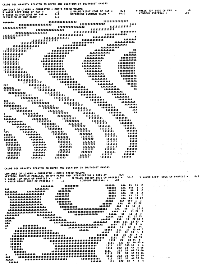
4-VARIABLE RELATIONS OIL GRAVITY, WELL DEPTH, GEOG LOC IN SE KANSAS
13 X 13 (X,Y) MATRIX VALUES

2.44,  02   5.69,  03   7.44,  02   9.73,  02   3.51,  03   2.27,  04   3.09,  03   1.48,  04   1.45,  05   5.26,  03   2.05,  04   3.87,  06   3.30,  04
5.69,  03   1.45,  05   1.48,  04   2.27,  04   6.07,  04   5.92,  05   5.67,  04   3.36,  05   3.87,  06   1.21,  05   3.16,  05   1.07,  08   7.45,  05
7.44,  02   1.48,  04   3.51,  03   3.09,  03   2.05,  04   5.67,  04   1.58,  04   6.07,  04   3.36,  05   1.77,  04   1.32,  05   8.20,  06   1.15,  05
9.73,  02   2.27,  04   3.09,  03   5.26,  03   1.58,  04   1.21,  05   1.77,  04   5.67,  04   5.92,  05   3.30,  04   9.67,  04   1.64,  07   2.25,  05
3.51,  03   6.07,  04   2.05,  04   1.58,  04   1.32,  05   2.40,  05   9.67,  04   3.16,  05   1.22,  06   9.73,  04   9.04,  05   2.73,  07   6.69,  05
2.27,  04   5.92,  05   5.67,  04   1.21,  05   2.40,  05   3.18,  06   2.97,  05   1.24,  06   1.64,  07   7.45,  05   1.30,  06   4.73,  08   5.02,  05
3.09,  03   5.67,  04   1.58,  04   1.77,  04   9.67,  04   2.97,  05   9.73,  04   2.40,  05   1.24,  06   1.15,  05   6.45,  05   3.02,  07   8.07,  05
1.48,  04   3.36,  05   6.07,  04   5.67,  04   3.16,  05   1.24,  06   2.40,  05   1.22,  06   8.20,  06   2.97,  05   1.89,  06   2.10,  08   1.80,  06
1.45,  05   3.87,  06   3.36,  05   5.92,  05   1.22,  06   1.64,  07   1.24,  06   8.20,  06   1.07,  08   3.18,  06   5.71,  06   3.03,  09   1.97,  07
5.28,  03   1.21,  05   1.77,  04   3.30,  04   9.73,  04   7.45,  05   1.15,  05   2.97,  05   3.18,  06   2.25,  05   6.26,  05   9.01,  07   1.61,  06
2.05,  04   3.16,  05   1.32,  05   9.67,  04   9.04,  05   1.30,  06   6.45,  05   1.89,  06   5.71,  06   6.26,  05   6.39,  06   1.16,  08   4.44,  06
3.87,  06   1.07,  08   8.20,  06   1.64,  07   2.73,  07   4.73,  08   3.02,  07   2.10,  08   3.03,  09   9.01,  07   1.16,  08   8.78,  10   5.70,  08
3.30,  04   7.45,  05   1.15,  05   2.25,  05   6.69,  05   5.02,  06   8.07,  05   1.60,  06   1.97,  07   1.61,  06   4.44,  06   5.70,  08   1.19,  07

1 X 13 COLUMN VECTOR VALUES


8.98,  03   2.11,  05   2.67,  04   3.56,  04   1.24,  05   8.42,  05   1.09,  05   5.39,  05   5.40,  06   1.93,  05   7.17,  05   1.45,  08   1.21,  06

EQUATION COEFFICIENTS
LINEAR, Z = 36.30596 + .0812557W + .3449529X + -.0900418Y

LIN + QUAD, Z = 37.90548 + .0662714W + -1.0362317X + -.6831682Y + -.03199614X2 + -.03304167WY + -.09474352XY

       + .03523953WX + .00094850W2 + .20109156Y2

LIN + QUAD + CUB, Z = 45.20266 + -.9616497W + -.3940345X + -4.3746648Y + -.01570835X2 + -.03085394WY

       + -.07620920XY + .01609525WX + .05903346W2 + 1.16790819Y2 + .00014462X3 + -.00093207W3+ -.07155833Y3

ERROR MEASURE LINEAR TREND SURFACE = 9.86
ERROR MEASURE QUADRATIC TREND SURFACE = 8.82
ERROR MEASURE CUBIC TREND SURFACE = 8.04
PERCENT TOTAL SUM SQUARES LINEAR SURFACE = 31.97
PERCENI TOTAL SUM SQUARES QUADRATIC SURFACE = 49.69
PERCENT TOTAL SUM SQUARES CUBIC SURFACE = 62.96
SUM OF SQUARES DUE LINEAR COMPONENT = 330624.23
SUM OF SQUARED DEVIATIONS FROM LINEAR = 2395.34
SUM OF SQUARES DUE LINEAR + QUADRATIC COMPONENT = 330876.85
SUM OF SQUARES DUE TO QUADRATIC ALONE = 252.62
SUM OF SQUARED DEVIATIONS FROM LINEAR + QUADRATIC = 2142.68
SUM OF SQUARES DUE LINEAR + QUADRATIC + CUBIC = 331065.94
SUM OF SQUARED DEVIATIONS FROM LINEAR + QUADRATIC + CUBIC = 1953.58
SUM OF SQUARES DUE CUBIC ALONE = 189.09
VOLUME WITHIN LINEAR SURFACE = 96579.17
VOLUME WITHIN LIN + QUAD SURFACE = 97826.04
VOLUME WITHIN LIN + QUAD + CUB SURFACE = 99533.01
ARITH. MEAN Z, = SUM OF Z VALUES/ N = 36.79
AVERAGE Z VALUE, LINEAR SURFACE = 35.87
AVERAGE Z VALUE, LIN + QUAD SURFACE = 36.33
AVERAGE Z VALUE, LIN + QUAD + CUB SURFACE = 36.96
VOL OF BLOCK IN CUBED UNITS = 2692.80

WCOORD   XCOORD   YCOORD    Z-VALUE   1ST-TRD   1ST-RSD   2ND-TRD  2ND-RSD   3RD-TRD    3RD-TRD
   19.0      6.1       .7       39.4      35.7      3.7       37.2      2.2      37.5        1.9
   18.1      7.9       .3       37.4      34.9      2.5       37.0       .4      37.6        -.2
   19.8      6.0      1.5       34.8      35.7      -.9       36.3     -1.5      35.3        -.5
   20.0      6.1      1.5       34.3      35.7     -1.4       36.3     -2.0      35.3       -1.0
   17.9      7.8       .7       36.6      35.0      1.6       36.9      -.3      36.5         .0
   15.2      8.0       .9       35.0      34.7       .3       35.6      -.6      34.8         .2
   17.3      7.5       .5       38.7      35.1      3.6       37.0      1.7      37.3        1.4
   16.5      7.4       .5       41.8      35.0      6.8       36.7      5.1      37.0        4.8
   18.0      7.0       .1       41.4      35.3      6.1       38.0      3.4      39.6        1.8
   25.0      4.3      1.7       38.5      36.7      1.8       37.4      1.1      37.0        1.5
   25.0      4.3      2.0       30.9      36.7     -5.8       37.1     -6.2      36.4       -5.5
   24.0      4.5      1.6       37.2      36.6       .6       37.3      -.1      36.9         .3
   23.5      4.5       .9       39.6      36.6      3.0       38.2      1.4      38.7         .9
   23.7      5.0       .8       40.7      36.4      4.3       38.4      2.3      39.1        1.6
   24.5      4.7      1.4       40.3      36.5      3.8       37.7      2.6      37.4        2.9
   22.0      5.3       .5       41.0      36.2      4.8       38.4      2.6      39.6        1.4
   21.0      5.5      1.7       33.6      36.0     -2.4       36.4     -2.8      35.4       -1.8
   22.5      5.4       .2       39.2      36.3      2.9       39.1       .0      41.2       -2.0
   23.0      5.5       .1       40.2      36.3      3.9       39.5       .7      41.9       -1.7
   19.1      6.2      2.3       30.3      35.5     -5.2       35.2     -4.9      33.6       -3.3
    7.8      6.4      3.3       30.8      34.4     -3.6       32.0     -1.2      31.8       -1.0
   19.5      6.4      3.0       26.6      35.4     -8.8       34.6     -8.0      33.1       -6.5
   12.3      6.4      3.4       35.7      34.8       .9       32.9      2.8      31.6        4.1
   34.7       .1      8.5       39.5      38.3      1.2       40.3      -.8      38.0        1.5
   37.6       .1      8.7       41.6      38.5      3.1       40.2      1.4      36.0        5.6

Part 2

Examples of contours drawn on sides of block intersecting third-degree hypersurface. Reference contour line is formed by edge of band of $ signs facing band of A's.

Part 3

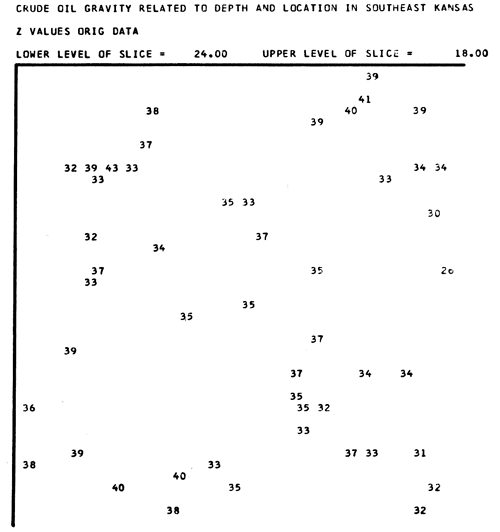
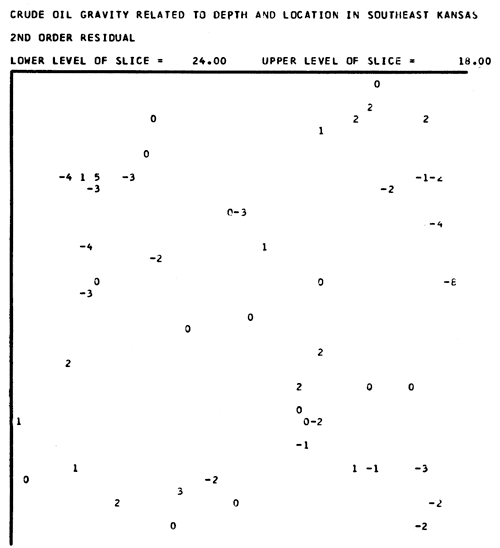
Examples of slice maps where data values have been plotted by computer. Map below contains original data values and following map contains second-degree residual values. Lines were added by band to show left and top boundaries of each map. Origin is in upper left corner of each map where lines intersect.

Prev Page--Start of Bulletin

Kansas Geological Survey, Oil-gravity Variations
Placed on web Jan. 25, 2012; originally published in 1964.
Comments to webadmin@kgs.ku.edu
The URL for this page is http://www.kgs.ku.edu/Publications/Bulletins/171/02_append.html