
 |
Original published in D.F. Merriam, ed., 1964, Symposium on cyclic sedimentation: Kansas Geological Survey, Bulletin 169, pp. 415-425 | |
University of Kansas, Lawrence, Kansas
It is the purpose of this paper to present some preliminary studies indicating how the methods of Fourier analysis might be used to identify and classify formations based on their electrical characteristics.
Periodicity is one of the fundamental phenomena recorded by observant man. Cycles associated with astronomical events were among the first natural phenomena described with sufficient precision and generality that such events could be predicted for the future. Even for primitive societies, one measure of their level of scientific understanding is the accuracy of their calendars.
Explanations of sound, tone, and harmonics were among the first elements of modern physical science. This early success in description and prediction of periodic astronomical events together with an understanding of periodicity related to vibration in the production of sounds led scientists to seek periodicities elsewhere in the natural world. Today the list is extensive for phenomena in which cycles have been studied. It includes sunspot activity, tides and ocean waves, earth tides, music, human speech, tree-ring growth, animal population changes, brain waves, heart rhythm, chemical bonding forces, climatic activity, economic growth, light and other electromagnetic wave phenomena, and geological events. The geological phenomena include varve growth and gross sedimentation trends in the sense of A. B. Vistelius (1961) as well as the more generalized cyclothems and megacyclothems of R. C. Moore (1936).
A common feature of the study of periodicity in natural phenomena is the search for the more important cycle periods or cycle frequencies. An attempt then is made to explain the cycles in terms of more fundamental phenomena.
The classic method of harmonic analysis involving Fourier series, has been used to determine these cycles. No general method exists for relating the detected cycles to other phenomena. Thus, although cycles seem to be apparent in the varve thickness sequences studied by Anderson and Koopmans (1963), no immediately obvious connection exists between these observed cycles and other cyclic phenomena, although such a relation undoubtedly exists.
Recently, a new approach has been taken to the study of oscillatory phenomena in which concepts of statistics have been applied to generalized harmonic analysis theory, allowing periodicities to be detected in the presence of noise. Noise is defined here as oscillation of the value of a variable without any periodicity. Thus, one may speak of the random variation of a variable. Where periodicities as well as the random variation are present in a variable, the cyclic component may be obscured unless some means is used to separate or filter out the "noise."
Figure 1 indicates the three types of variation (a) periodic, (b) random, and (c) combined periodic and random. The variable on the vertical scale might represent, for example, tree-ring width, varve thickness, an economic index such as gross national product, an electronic signal, or height of water in a basin subject to wave action.
Figure 1--Types of oscillitory behavior: (a) periodic oscillation, (b) random oscillation devoid of periodic component, and (c) composite oscillation, containing periodic and random fluctuations.
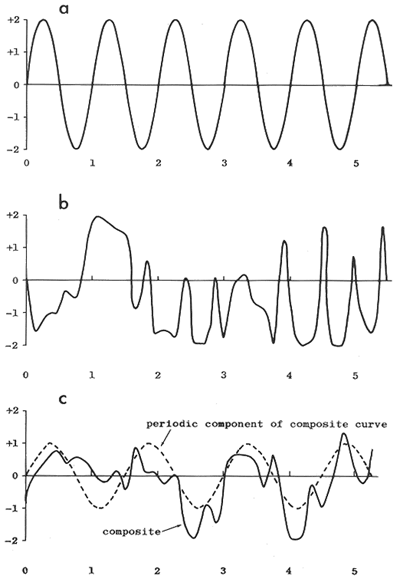
Most phenomena that are observed to be oscillatory seem to possess both random (noisy) and periodic components. Methods for separating noise from periodic signals are now reasonably developed within the field of electrical communication. Much of the theory is directly applicable in other disciplines. Even with the application of these new methods, it is not always possible to completely separate the desired periodic portion from the noise. However, the generalized theory of harmonic analysis makes it possible to quantitatively represent a particular sample of a composite periodic signal and the noise to any desired degree of accuracy. This combined oscillatory signal represents only the observed portion of the phenomenon and not the totality of the separate periodic and random components. In a sense, one may say that this sample of the combined signal contains all the available information on the phenomenon, assuming no other samples are available. What is desired is some minimal set of numbers to represent this signal sample. The set of numbers should be minimal in the sense that it takes fewer of them to represent the signal than the original signal contained. It will be shown that through Fourier analysis such a set of numbers is extractable for a given signal and that under the proper circumstances, this set of numbers is an appropriate descriptor of the phenomenon; that is, the number set can be used to distinguish members of one class from those in another class (Henderson, 1962).
Acknowledgements--We wish to thank Dr. Daniel F. Merriam for assistance in selection and analysis of the electric logs and for construction of the geologic cross sections. Calculations were performed on an IBM 650 computer under a grant from The University of Kansas Computation Center. Mr. W. B. Tjokronegoro assisted in the preparation of the figures and Dr. John W. Harbaugh kindly reviewed the manuscript.
One may consider an electric log to represent resistivity or some other electrical property averaged over a short distance. A common feature of these logs is their oscillatory character. Although gross changes in pattern can be correlated with known changes in lithology, all too frequently, the detail of the oscillatory signal in the resistivity log in a long undifferentiated shale sequence, for example, contains more information than can be used in a simple stratigraphic classification. Furthermore, a simple picture matching will frequently indicate a lack of correspondence on a detailed scale between logs in adjacent wells penetrating this undifferentiated sequence. Sections of this type are most frequently identified by abrupt and easily recognizable changes that mark their upper and lower boundaries rather than by any characteristic of their interior region. It is believed that Fourier series may represent a means for characterizing sections of logs that have a rather complex logged structure and yet are relatively featureless when viewed by conventional "picture matching" methods.
The Fourier series is given by

where L = half of the basic or fundamental period; in applications where this is not known, it may be taken as half the length over which a signal is sampled
z = the independent variable of length along the well bore, wherein -L ≤ z ≤ L
a0 = the zeroth coefficient of a
an = the maximum value (or amplitude) of the cosine term
![]()
![]()
y = the dependent variable, such as resistivity, taken to be a function of length or distance z, along the well bore.
Equation (1) represents a summing of a large number (in the limit this is infinite) of individual pure sine and pure cosine waves, each with its own period, (2L/n), and amplitude (an for cosines and bn for sines). If appropriate values for the amplitudes (also called coefficients) are chosen, then, with certain exceptions which we shall not consider here, one may represent a large class of oscillatory and some nonoscillatory curves to any desired accuracy.
Because one does not know the mathematical equation of the electric log signal, to represent electric logs as a series of sine and cosine terms, one must use a finite and usually small number of terms (less than 30) in the series (Table 1). Thus, one may represent a resistivity or other log to any desired accuracy by equation (1) assuming a sufficiently large number of points and terms is chosen for the series.
Table 1--Observed and computed resistivities for O.A. Sutton No. 1 Gish well. Refer to Figure 1 for location.
| Point no. |
Index | Observed resistivity, ohm-meters |
Computed resistivity, ohm-meters |
|---|---|---|---|
| 1 | -12 | 9.10 | 16.34 |
| 2 | -11 | 28.80 | 28.98 |
| 3 | -10 | 54.80 | 53.94 |
| 4 | -9 | 58.50 | 58.68 |
| 5 | -8 | 61.00 | 60.14 |
| 6 | -7 | 66.00 | 66.18 |
| 7 | -6 | 15.65 | 14.79 |
| 8 | -5 | 28.90 | 29.08 |
| 9 | -4 | 57.00 | 56.14 |
| 10 | -3 | 81.00 | 81.18 |
| 11 | -2 | 81.00 | 80.14 |
| 12 | -1 | 14.00 | 14.18 |
| 13 | 0 | 54.00 | 53.14 |
| 14 | 1 | 65.00 | 65.18 |
| 15 | 2 | 57.50 | 56.64 |
| 16 | 3 | 65.00 | 65.18 |
| 17 | 4 | 33.00 | 32.14 |
| 18 | 5 | 31.00 | 31.18 |
| 19 | 6 | 32.40 | 31.54 |
| 20 | 7 | 37.45 | 37.63 |
| 21 | 8 | 17.60 | 16.74 |
| 22 | 9 | 15.80 | 15.98 |
| 23 | 10 | 24.10 | 23.24 |
| 24 | 11 | 26.30 | 26.48 |
| 25 | 12 | 17.20 | 16.34 |
For the case in which the mathematical equation of the "signal" is not available, the method for determining the set of coefficients an and bn is known as harmonic analysis and is described in standard texts on Fourier series (Scarborough, 1962; Lancios, 1961; Gaskell, 1958) . The coefficients are determined from the following equations:
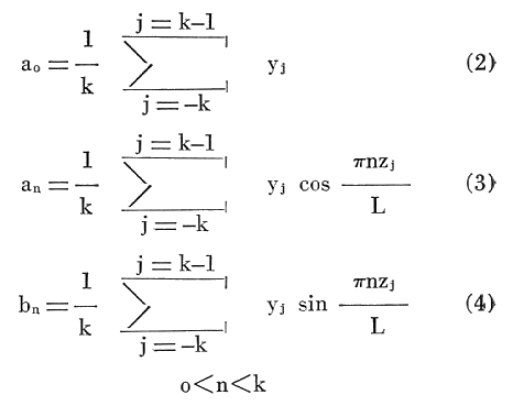
where Yj = the measured resistivity or other logged property at the point j in the interval from -L to +L
j = an index denoting the j'th value of y; an odd number, 2k + 1, of equally spaced points is chosen in the interval -L to +L. The points are numbered from -k to +k at intervals of 1
k = the number of equal width panels in the interval 0 to L.
It can be shown that the coefficients obtained by equations (2), (3), and (4) satisfy the least-squares criterion, in that the sum of the squares of the deviations of the predicted values, equation (1), from the observed values is a minimum. Thus, harmonic analysis can be considered to be a special case of polynomial regression or polynomial curve fitting, using a periodic function as the polynomial.
It may be shown (Wylie, 1951) that cn defined as
![]()
is a measure of the contribution made by the n'th harmonic to the total function, equation (1). The group of numbers, c12, c22, c32, . . . , cn2, constItutes a discrete spectrum or set and, by analogy to the concept of electrical power in alternating circuits theory, is called the power discrete spectrum of the function given by equation (1). More important, whereas the values of an and bn are dependent upon the location of the section in a continuous oscillating signal from which the length -L to +L is chosen, the values of cn are independent of this location, assuming 2L is the fundamental period of the signal. Thus, although the sets of coefficients, an and bn could be used to characterize an otherwise undifferentiated section, it was considered that the set cn would generally be more amenable to correlation from well to well.
For this study, the Lansing Group, consisting of alternating limestone and shale beds in eight wells in Butler and Cowley Counties, Kansas, was studied by harmonic analysis. After picking the top and bottom of the group, the record of the logged section was enlarged photographically and the interval was divided into 24 panels by a set of 25 equally spaced points. The fundamental period was arbitrarily taken as 24, and the coefficients an, bn, and cn were determined for the first twelve harmonics, i.e. n = 12 (Table 2). The resistivity (short normal) log profiles in this area are shown in Figure 2, and the corresponding power spectra are given in Figure 3. These line spectra can be considered as a type of transformed resistivity log. Adjacent wells can be compared for similarity by comparing their power spectra, similarity of resistivity logs being synonymous with similarity of power spectra. Wells 6 and 7 penetrate a marine limestone bank and are noticeably different, particularly as regards their c1 and c2 components.
Table 2--Harmonic coefficients for Fourier-series analysis of resistivity log for O. A. Sutton No. 1 Gish well.
| Harmonic n |
Cosine term an |
Sine term bn |
Cn |
|---|---|---|---|
| 0 | 42.28750 | ||
| 1 | 13.05240 | -10.26861 | 16.60751 |
| 2 | 1.85156 | 7.65094 | 7.87180 |
| 3 | 1.86623 | -4.95496 | 5.29476 |
| 4 | -12.11042 | 0.76860 | 12.13148 |
| 5 | -7.97458 | 10.79408 | 13.42035 |
| 6 | -2.13750 | 4.78750 | 5.24300 |
| 7 | 6.45539 | 2.79072 | 7.03280 |
| 8 | -0.18124 | 2.52952 | 2.53600 |
| 9 | 2.36709 | 6.87004 | 7.26639 |
| 10 | 6.07344 | 3.81156 | 7.17039 |
| 11 | 2.63346 | 1.18475 | 2.88769 |
| 12 | -1.04167 | 0.00000 | 1.04167 |
Figure 2--Resistivity log profile for Lansing Group (Pennsylvanian). Well 1, Saturn No. 1 Stone--NW NW NE sec. 23, T. 24 S., R. 7 E. Well 2, Sutton No. 1 Gish--NW NW SE sec. 12, T. 25 S., R. 7 E. Well 3, Kewanee No. 1 Ferry--NE NE NW sec. 12, T. 26 S., R. 7 E. Well 4, Gross No. 7 Steward--C E2 E2 SW SW sec. 12, T. 27 S., R. 7 E. Well 5, Holley No. 27 Ferrell--NW NE SE sec. 21, T. 28 S., R. 8 E. Well 6, Gralapp and Everly No. 1 Ellis--SW SW SW sec. 25, T. 29 S., R. 7 E. Well 7, Marts No. 1 "A" Smith--C E2 NW SW sec. 28, T. 30 S., R. 7 E. Well 8, Royal No. 1 Fox--SW SW SE sec. 15, T. 31 S., R. 7 E. A larger version of this figure is available.
Figure 3--Power spectra for Lansing Group wells shown in Figure 2: (1) Saturn No. 1 Stone; (2) Sutton No. 1 Gish; (3) Kewanee No. 1 Ferry; (4) Gross No. 7 Seward; (5) Holley No. 27 Ferrell; (6) Gralapp & Everly No. 1 Ellis; (7) Marts No. 1 "A" Smith; (8) Royal No. 1 Fox. A larger version of this figure is available.
A similar power-spectrum analysis was made of alternating limestone and shale beds in the Lansing Group in four wells in Phillips County, Kansas. A fifth well (Fig. 4, well 5) was used as a control wherein an interval in the Kansas City Group similar to the Lansing interval was purposely used for the power-spectrum analysis. Logs are shown in Figure 4 and power spectra in Figure 5. Although several types of differences may be distinguished in the five power spectra of Figure 5, a basic difference between the spectra of wells 1 through 4 and that of well 5 is the reversal in the relative magnitudes of the c1 and c2 components. This apparent uniqueness of the spectrum of well 5 was also confirmed by the discriminant-function analysis.
Figure 4--Resistivity log profile for Lansing Group in north-central Kansas. Well 1, Sohio No. 2 Krause--NW SE SE sec. 1, T. 4 S., R. 19 W. Well 2, Carter No. 1 Vogel--C NE SW sec. 26, T. 3 S., R. 19 W. Well 3, Imperial No. 3 Vogel--SE NE NE sec. 14, T. 3 S., R. 19 W. Well 4, Prugh No. 1F Jackson--SW SE SW sec. 21, T. 1 S., R. 19 W. Well 5, Westgate Greeland No. 1 Roland--SW SW SW sec. 21, T. 1 S., R. 17 W. A larger version of this figure is available.
Figure 5--Power spectra for logs of Figure 4: (1) Sohio No. 2 Krause; (2) Carter No. 1 Vogel; (3) Imperial No. 3 Vogel; (4) Prugh No. 1F Jackson; (5) Westgate Greeland No. 1 Roland. A larger version of this figure is available.Although it is valuable to have a means of condensing and representing resistivity measurements of logs in a transformed mode, the primary utility of harmonic analysis is that it yields a set of numerical coefficients which can be considered as a multidimensional description of the original log, allowing analysis by conventional statistical methods. One such method employs the discriminant function. In instances in which classification has been previously established, this technique is useful for identifying an unknown individual record as being from one particular class.
An early reference (Barnard, 1935) concerning the discriminant function deals with an analysis of variations in skull characteristics. It seems that R. A. Fisher conceived the technique and suggested it to Barnard. Explanations of the method and suggestions for practical use may be found in Kendall (1946), Keeping (1962), and Bennett and Franklin (1954).
The use of the discriminant function may be illustrated as follows: Suppose that n individuals are known to be from one population and m individuals are known to be from another population. For each of these individuals we observe a number of characteristics x1, x2, . . . , xk. What linear combination of these k characteristics,
X = a1x1 + a2x2 + . . . + akxk (6)
will best reflect the difference between the two populations? The term X, defined to characterize this difference, is the discriminant function.
It is assumed that for each population, the k characteristics have a multivariate normal distribution, with different means but common variances and covariances. The effect of departure from the assumption of common variances and covariances is not discussed in the literature. Fisher and others do not test for, or mention the effect of, the assumption.
From n observations on k characteristics of the first population, the means for each characteristics, ![]() 1,1,
1,1, ![]() 1,2,
1,2, ![]() 1,k, and the matrix of the sums of squares and cross products of deviations from the mean may be found:
1,k, and the matrix of the sums of squares and cross products of deviations from the mean may be found:
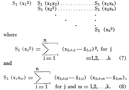
The means and the matrix for the k characteristics of the m individuals in the second population may be found in a similar fashion. From the k means of the characteristics from the two populations one may obtain the esti. mate of their differences
![]()
The matrix of the joint estimates of the common variances and covariances,
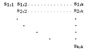
may be found using
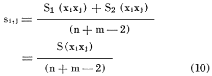
The difference, D, of the means of X for the two populations can be found from
![]()
The variance of X based on the variations within the two populations can be estimated from

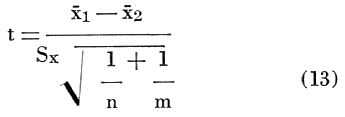

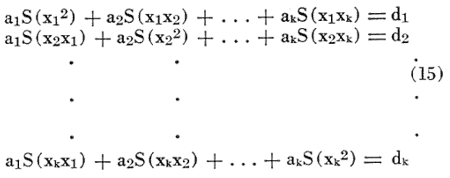
accomplish this purpose.
Because the problem is to assign a sample of unknown origin to one of the two parent populations (or to neither), the "t" test on the value from equation (14) is of no value.
Recalling from equation (12) that Sx represents an estimate of the standard deviation of the X's, one can measure the strength of the discriminant function. The value of D/Sx gives the number of standard deviations separating the means of the X's for the two populations. As the X's are assumed to be normally distributed, random variables with the same standard deviations, they can be represented by identical probability density function curves with different means. Ideally, it would be desirable to have no overlap of the two curves. However, as the curves are asymptotic as X tends to plus or minus infinity, they will always overlap to some extent. One can consider the discriminant function a good one if this area of overlap is very small. As an example, if the two probability density function curves have means which are 6Sx apart, they will intersect at -3Sx on the curve for the population with the greater mean and + 3Sx for the other. The area under the standard normal curve from 3Sx to infinity is .0013. Therefore, the probability of assigning a sample to the first population when it belongs in the second is .0013, and vice versa.
To assign the sample to the proper parent population, the limits x ± bSx are chosen so that bSx is less than the distance from the mean, x, to the area of overlap for each population. Thus, if the value of X for the sample falls within the limits ![]() ± bSx for one of the populations, the sample is assigned to that population. If it falls outside these limits, the sample probably did not come from either population. If it falls within the area of overlap, no safe decision can be made.
± bSx for one of the populations, the sample is assigned to that population. If it falls outside these limits, the sample probably did not come from either population. If it falls within the area of overlap, no safe decision can be made.
In this analysis, the coefficients, cn, obtained by harmonic analysis were taken as the measurements x1, x2, x3, . . . , Xk. The first four logs of the Lansing Group of Figure 4 and the eight Lansing Group sections shown in Figure 2 were taken as populations 1 and 2 respectively. The first seven elements of the spectral series, cn, for each population were chosen as the characteristic measurements, x1, x2, x3, . . . , Xk. The discriminant function for these two populations was:
X = .12989c1 - .21221c2 - .16497c3 - O2864c4 + .16856c5 + .27108c6 - 34991c7 (16)
Using the average values of cn for each population, one obtains ![]() 1 = .386 and
1 = .386 and ![]() 2 = -3.908 with Sx = .596.
2 = -3.908 with Sx = .596.
The strength of the discriminant function may be found from

Thus, the probability density functions for the two populations will overlap at ![]() 1 - 2.95 Sx and
1 - 2.95 Sx and ![]() 2 + 2.95 Sx. The area under the curve at a distance of 2.95 Sx from the mean is .0016. The probability of classifying the unknown well in one population when it should be in the other is therefore .0016. In other words, there are 9,984 chances out of 10,000 that the proper classification will be made.
2 + 2.95 Sx. The area under the curve at a distance of 2.95 Sx from the mean is .0016. The probability of classifying the unknown well in one population when it should be in the other is therefore .0016. In other words, there are 9,984 chances out of 10,000 that the proper classification will be made.
With such a powerful discriminant function, one can conservatively choose the limits ![]() ± bSx at
± bSx at ![]() ± 2.5Sx. Using these limits, one may say that if the value
± 2.5Sx. Using these limits, one may say that if the value ![]() calculated from equation (16) using the Ci from an unknown sample falls in the range -5.398 to -2.418 the well is more nearly similar to the Lansing Group of cross section B than of cross section A. If it falls in the range -1.876 to +1.104, the reverse is more likely to be true.
calculated from equation (16) using the Ci from an unknown sample falls in the range -5.398 to -2.418 the well is more nearly similar to the Lansing Group of cross section B than of cross section A. If it falls in the range -1.876 to +1.104, the reverse is more likely to be true.
To indicate how this classification process might be applied in a specific instance, the Kansas City Group (hatched section) of well 5 in Figure 5 was used as an unknown. The first seven members of the spectral series, cn, were obtained and using the values for en in equation (16), X was computed as -6.640. This value is shown in Figure 6 with the probability density function for the two mean values of X corresponding to populations 1 and 2. In this specific instance, as was to be expected, the formation did not fall into either classification.
Figure 6--Probability density functions for discriminant X when used to distinguish Lansing Group in two different regions. A larger version of this figure is available.
Preliminary studies presented herein indicate that Fourier analysis can be used to develop a set of numerical parameters that give a reasonably accurate representation of the electric log of a formation and that these parameters may be studied for periodicities. They also may become input data for statistical methods of formation correlation. A new use of Fourier analysis is herein proposed, namely the statistical, numerical characterization of a formation from its electric log and also assignment of a sample of unknown origin to one (or neither) of two parent populations based upon the derived numerical parameters. Methods for determining the strength of the discriminant function and the criterion for making the assignment were also outlined.
An example showing the use of the discriminant function to determine whether or not electric log data came from one of two known formations was presented. This example illustrated use of the methods for obtaining coefficients of the function and application of the decision criterion.
Additional applications of the discriminant function in the petroleum industry include: (1) drawing inferences as to the productive capacity of a well or reservoir based upon the known capacity of another well or reservoir to which it is similar, and (2) aid in reaching decisions concerning the relative effectiveness of various well stimulation processes.
Anderson, R. Y., and Kopmans, L. H., 1963, Harmonic analysis of varve time series: Jour. Geophysical Res., v. 68, no. 3, p. 877-893.
Barnard, M. M., 1935, The secular variations of skull characteristics in four series of Egyptian skulls: Annals Eugenics, v. 6, p. 352-371.
Bennett, C., and Franklin, N., 1954, Statistical analysis in chemistry and the chemical industry: Wiley & Sons, New York, p. 288-295.
Gaskell, R. E., 1958, Engineering mathematics: Holt, Rinehart, and Winston, Inc., New York, p. 191-225.
Henderson, J. H., 1962, Application of certain techniques of statistical inference to petroleum engineering: Unpub. master's thesis, Kansas Univ., 107 p.
Keeping, E. S., 1962, Introduction to statistical inference: Van Nostrand, Princeton, N. J., p. 366-371.
Kendall, M. G., 1946, The advanced theory of statistics, v. 1; Charles Griffin and Co., London, p. 341-348.
Lanczos, C., 1961, Applied analysis: Prentice Hall, Englewood Cliffs, N. J., p. 207-299.
Moore, R. C., 1936, Stratigraphic classification of the Pennsylvanian rocks of Kansas: Kansas Geol. Survey Bull. 22, 256 p. [available online]
Scarborough, J. B., 1962, Numerical mathematical analysis, 5th ed.: John Hopkins, Baltimore, p. 558-575.
Vistelius, A. B., 1961, Sedimentation time trend functions and their application for correlation of sedimentary deposits: Jour. Geology, v. 69. p. 703-728.
Wylie, C. R., Jr., 1951, Advanced engineering mathematics: McGraw-Hill, New York, p. 129-130.
Kansas Geological Survey
Comments to webadmin@kgs.ku.edu
Web version Feb. 2003. Original publication date Dec. 1964.
URL=http://www.kgs.ku.edu/Publications/Bulletins/169/Preston/index.html