Kansas Geological Survey, Bulletin 127, pt. 2, originally published in 1957
Originally published in 1957 as Kansas Geological Survey Bulletin 127, pt. 2. This is, in general, the original text as published. The information has not been updated. An Acrobat PDF version (4.8 MB) is also available.
Simple and rapid solutions of complex ground-water flow problems are desirable, Known analogies with fluid flow offer a means to overcome difficult problems with relatively little effort. A potentiometric model called a conducting-paper analog field plotter was chosen to utilize the analogy between fluid flow and electric current conduction. Electrical theory and model experiments show that the plotter cannot be applied accurately to any three-dimensional, steady-state, ground-water flow problems, Two-dimensional studies can be accomplished readily with the plotter, but other devices will have to be utilized for radial flow problems.
Increased use of ground water in the last few decades has made it necessary to develop methods of studying ground-water flow in various simple and complex situations. Ground-water flow theory permits relatively simple solutions when the flow system is confined to known geometrical figures and when certain assumptions are made. Natural conditions cause flow systems to develop proportions that are extremely difficult, if not impossible, to treat analytically. In difficult cases, analogies with other phenomena may prove useful.
Prior to the turn of the century it was known that electric current conduction is analogous to electrostatics, magnetostatics, and heat conduction (Maxwell, 1904). In other words, the phenomena have a common bond in the Laplace equation. C. S. Slichter (1899), in his classic paper Theoretical Investigation of the Motion of Ground Waters, showed that the flow of fluids is also analogous to the flow of electric current, flow of heat, etc. Since that time various devices have been constructed to employ this analogy.
A brief description of four main types of devices follows. Large electronic analog computers are capable of handling most flow variables, provided that the necessary properties of fluid and porous media are known. The equipment is costly and complex and requires experienced personnel for operation (Liebmann, 1953).
Another satisfactory method for solving flow problems is the resistor grid, which comprises a simple electrical system composed of numerous resistors arranged in a grid. Each resistor is adjusted and the voltage drop is measured across each resistor until the grid voltage matches the hydrologic data. The entire grid network will then simulate the flow problem in steady state. The apparatus is not expensive, and the tedious job of adjusting the resistors may be accomplished by relatively inexperienced personneL This method is well described by Luthin (1953) and Liebmann (1950).
A third device employing the fluid-electric flow analogy is the electrolytic tank model. The thickness of the electrolyte can be varied to reproduce the saturated medium. An electric current is passed through the solution between its boundaries, and equipotentials are plotted with a probe. In such a way, two- and three-dimensional plots may be constructed. This type of model has won some favor in petroleum industry research laboratories for use in studying the effect of flooding and other two-phase problems (Botset, 1945; Mason, 1954). Although primarily used in oil recovery work, an electrolytic tank model can be applied to ground-water problems where there are variations in the thickness and permeability of the aquifer. There are many thorough discussions on the theory and applications of the electrolytic model (Lee, 1947; Wolf, 1948; Bruce, 1943). Although models may take on elaborate proportions, they are basically inexpensive and relatively simple to operate.
The fourth device is the conducting-paper analog field plotter, which is similar to the electrolytic tank model except that the electrolyte is replaced by graphite-impregnated paper. It is this type of analog device that is discussed herein.
The conducting-paper plotter is inexpensive, is readily set up, and may be operated by inexperienced personneL There is no chance for shock or for spilling of an electrolyte solution. The resistance of the paper is constant and may be considered uniform. The main disadvantage is that only two-dimensional flow problems may be studied, as the plotter does not take into account variations in the vertical axis.
This work is the result of a suggestion by F. C. Foley, Director of the State Geological Survey of Kansas, and V. C. Fishel of the U. S. Geological Survey to consider the applicability of the plotter to ground-water problems. The analog plotter, together with incidental materials, and pumping data were furnished by the U. S. Geological Survey and the State Geological Survey of Kansas. Considerable plotting showed that theoretical and actual data from pumping wells would not yield satisfactory results. Discussion with C. F. Weinaug of the Petroleum Engineering Department and Daniel Ling of the Physics Department, University of Kansas, confirmed that results would be in error if the plotter were used to solve radial or gravity three-dimensional problems.
In many instances one physical phenomenon can be described in terms of another. Such an analogy can be established between Darcy's law and Ohm's law in a steady-state situation, and it is on this principle that the conducting-paper field plotter operates.
In simple form, Darcy's law states that the overall velocity of a fluid flowing through capillary interstices is directly proportional to the pressure gradient. Analytically, Darcy's law may be written as:
v=ph (1)
where v is the velocity, h is the difference in head per unit length (pressure gradient), and p is a constant of the porous medium (permeability).
Ohm's law may be expressed as:
I=V/R (2)
where V is the potential (volts), I is the current (amperes), and R is the resistance (ohms).
One may note that equations 1 and 2 have the same empirical form. Hence, an analogy may be made between the velocity of water and the electrical current, between the hydraulic head and the electric potential, and between the permeability and the reciprocal of the electrical resistance (Muskat, 1937).
If the fluid is incompressible, then the continuity equation for fluid flow becomes
(δvx / δx) + (δvy / δy) + (δvz / δz) = 0 (3)
Similarly, if the electric current is steady, then the continuity equation becomes
(δIx / δx) + (δIy / δy) + (δIz / δz) = 0 (4)
where vx, vy, and vz are velocity components and Ix, Iy, and Iz are electric current components in the x, y, and z directions respectively. [Note: Not only are equations 1 and 2 equivalent but also the continuity equation assumes the same form in the two situations.]
Darcy's law may be expressed as
v = -p (δh / δs) (5)
and Ohm's law as
I = -δV / (Rδs) (6)
In Darcy's law, if the vector s, the distance along the direction of flow, is resolved into three component vectors parallel to each of the axes in a Cartesian coordinate system (Jacob, 1950, p. 327), then
vx = -p (δh / δx)
vy = -p (δh / δy) (7)
vz = -p (δh / δz)
Similarly, for Ohm's law
Ix = (-δV / Rδx)
Iy = (-δV / Rδy) (8)
Iz = (-δV / Rδz)
Substituting the terms from either 7 or 8 into equations 3 and 4 and cancelling the constant terms results in
(δ2φ / δx2) + (δ2φ / δy2) + (δ2φ / δz2) = 0 (9)
where φ is the head, h, in the hydrodynamic system or the electrical potential, V, in the electrical system.
Equation 9 is the Laplace equation and must be satisfied by all steady-state flow problems. Slichter (1899) was the first writer to recognize that the Laplace equation holds for fluid flow.
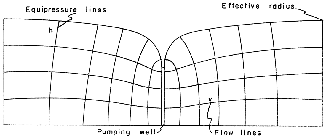
Slichter also included a proof that the flow path of a particle of water will, at all points, be normal to the line of equal hydraulic head. By convention, the flow lines will be spaced a distance apart equal to the distance between the equipotential lines and consequently will form squares. These squares are actually curvilinear squares having four right angles and equal mean distances between the opposite sides. If the curvilinear squares are repeatedly subdivided, a true square is approached (Taylor, 1948).
Figure 1 shows, in the profile of a pumping well, a simple ideal flow net consisting of lines of equal hydraulic head, h, and orthogonally plotted flow lines, v.
Figure 1—Profile through pumping well showing simple flow net consisting of lines of equal hydraulic head, h, and orthogonally plotted flow lines, v.
A steady-state flow toward a well must exist in order to apply the analogy between electric current and the flow of water in a porous medium. When no further drawdown occurs, the cone of depression is considered to be in equilibrium and a steady state of flow exists.
A formula, developed from Darcy's law by Thiem (1906), may be used to determine permeability once data are obtained from a cone of depression in equilibrium. For water-table and artesian conditions, the Thiem formula may be written
p = [Q (loge r2 - loge r1)] / [2 m (s1 - s2) (10)
where P is the coefficient of permeability, Q is the discharge from the well, r1 and r2 are distances from the pumped well to the respective points of observation, s1 ands2 are the drawdowns at the respective observation wells, and m is the average thickness of the saturated portion of the water-bearing material at the observation wells (Wenzel, 1942). If r1 and r2 are plotted on the logarithmic scale of semilogarithmic paper against s1 and s2 on the arithmetic scale, the straight line joining these two points will also pass through any other points determined by additional observation wells. For use in connection with the semilogarithmic paper, equation 10 is modified by converting the natural logarithms to common logarithms. If the discharge from the well is expressed as gallons per minute, q, then
p = (527.7 q) / (m Δs) (11)
where Δs is the drawdown over one logarithmic cycle on the semilogarithmic paper. From equation 11 the permeability in a steady-state condition can be determined.
In summary, Darcy's law and Ohm's law were shown to lead to the Laplace equation. Hence, an analogy exists between them. In a steady-state situation, plotting s against r on semilogarithmic paper results in a straight line.
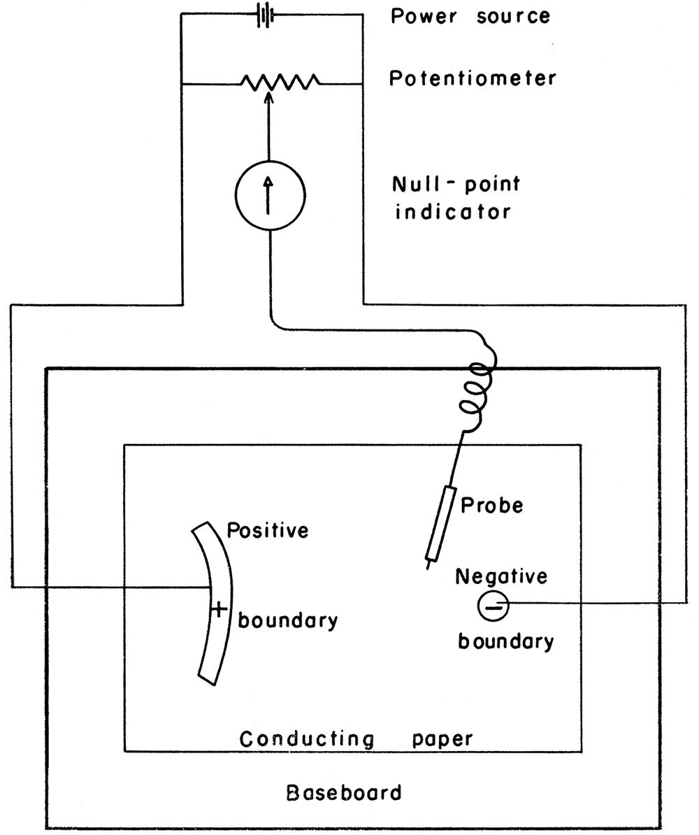
The conducting-paper type of analog plotter consists of seven essential units (Pl. 1). Each of the parts will be discussed in detail. Much of the discussion in this section is based on information contained in the manufacturer's manual, Use and Theory of the Analog Field Plotter. The equipment was obtained from the Sunshine Scientific Instrument Company, Philadelphia, Pennsylvania. A similar device can be constructed from materials available commercially. Figure 2 shows the wiring diagram for an analog field plotter.
Plate 1—Analog field plotter showing power unit and voltage divider, null-point indicator, probe, conducting paper, baseboard, and boundary materials.
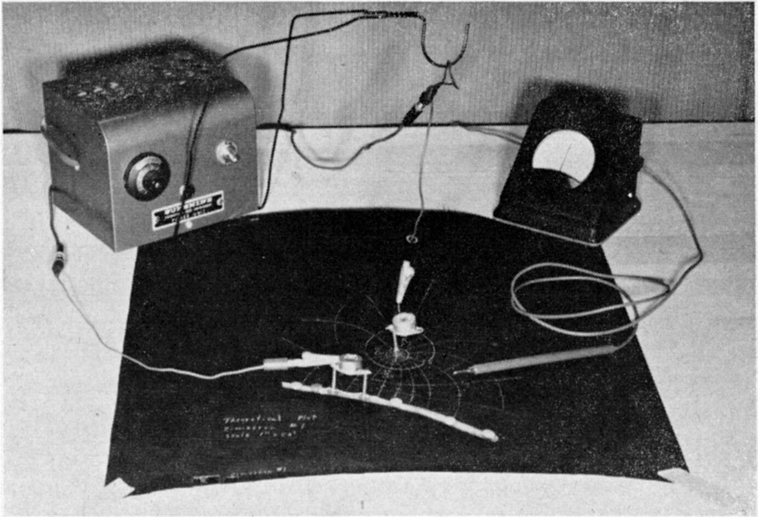
Figure 2—Schematic wiring diagram of analog field plotter circuit using a battery power source.
The power unit consists of a transformer, a selenium rectifier, an off-on toggle switch, overload fuses, and a tell-tale red light. The transformer and rectifier are the same as those found in most automobile battery chargers.
The transformer receives a 120-volt, 60-cycle alternating current and reduces the voltage to about 7 volts. The selenium disk dry rectifier converts the current from alternating to direct and is capable of supplying 5 amperes or more. As the plotter operates on a very low current, measured in milliamperes, the current supply from the rectifier is more than sufficient. The transformer and the rectifier are fused against external short circuits. A telltale lamp shows when the unit is in operation. The off-on switch is a single-throw, single-pole toggle switch connected to one side of the input power line. There are many uninsulated connections within the power unit. Consequently, the power unit must not be energized when the cover is open because a short circuit could result.
A 6-volt dry cell battery could be used equally well for a supply source.
The voltage divider, or potentiometer, is the type manufactured under the trade name "Helipot". On a ten-turn helical-wound resistance element, the arm ("slider") moves the complete length of the helix on a ten-turn screw. Position of the arm is indicated on a double dial (trade name "Duodial"), which has 100 units on an inner dial and 10 units on an outer dial. In this manner the voltage is divided into 1,000 separate readable units. The three posts on the back of the power and voltage divider unit are leads from the voltage divider. The center post, leading from the "slider", is connected to one post on the null-point indicator. The leads from the selenium rectifier are connected to the other two posts and complete the circuit.
The null-point indicator is a sensitive moving-coil microammeter, which detects a point of zero flow when the probe is located at a point on the paper where the potential is balanced by the setting on the voltage divider. In other words, the meter indicates zero potential in a _ potentiometric circuit. The meter face has a zero center and a ten-unit scale on each side of the center. The base of the meter is insulated to permit the meter to be placed on the conducting paper. A desirable feature in the meter is an overload shunt circuit consisting of two germanium diodes that prevent a severe surge of current from damaging the meter. When the current flow is low, only a very small percentage of the current is shunted through the diodes. If, by accident, the probe should be placed at a point far from an equipotential line (according to the setting on the voltage divider), the needle on the meter will go off the scale, but almost all of the current will be shunted around the needle mechanism. Oversensitivity is prevented by damping so that the null-point indicator gives the same reading within a plus or minus O.Ol-inch movement of the probe under normal reading conditions. As the null-point detector operates on extremely small current, no appreciable distortion is caused in the field pattern by the contact of the probe. Variation in voltage will not affect the operation of the null-point indicator, because it is recording a zero voltage. Should the needle, for any reason, fail to read zero when there is no current flowing through the meter, the needle can be reset by a small screw below the face of the dial. The two posts on the back of the meter are connected with the center post of the power unit and with the lead to the probe.
The probe, also called the searching and marking stylus, is connected to the null-point indicator by a long flexible wire. It is a sharp-pointed brass rod used to locate the equipotential points and to indent the paper at these points. The brass rod is insulated from the hand by a plastic sleeve. When a series of equipotential points has been determined by the probe, the indentations are connected by a colored pencil or white ink to indicate an equipotential line. With a new setting on the voltage divider, repetition of the process gives a trace of another equipotential line at a known drop in potential. It is not necessary to perforate the paper in order to mark it, as slight indentation suffices. If the paper is perforated, however, the current distribution pattern will not be appreciably altered.
The special conducting paper, made under the trade name of "Type L Teledeltos" paper, is of carbon-impregnated stock. It is manufactured in rolls 31 inches wide and 100 or 200 feet long. The resistance is constant throughout and has a value of 4,000 ohms per square, each square having the same ohmic resistance irrespective of size. The resistance in the paper is sufficiently uniform so that it may be considered analogous to a homogeneous aquifer. Manufacturing tolerance is plus or minus 8 percent along the length of the roll and plus or minus 3 percent along the width of the roll. These tolerances are within the realm of accuracy achievable for ground-water plots. Variations can be detected readily if the probe indentations are close enough, and irregularities can be overcome by drawing a smooth curve through the points. There is no satisfactory method yet known to vary the resistance in a portion of the paper by any controlled amount. Either the black or the silver side of the paper may be used for plotting.
Clearly, a nonconducting material should underlie the paper. Any wooden drawing board of sufficient size is acceptable. In order to make a plot 8 1/2 x 11 inches, the paper should be cut two to three times larger in order to make unbounded areas appear infinite with respect to the problem. Unless bounded by electrodes (painted boundaries), the field will extend to the limits of the paper even though the values of the equipotential lines may be low enough to be regarded as negligible. A pantograph can be used with the plotter to duplicate the field on a plain sheet of paper. As an alternative, carbon paper may be placed over a plain sheet of parer under the plot when the equipotential and flow lines are drawn. The latter method is considerably easier for one person to handle.
In order to control the circuit across the conducting paper, boundaries of low resistance must be inserted. The great difference between the resistance of the paper (4,000 ohms per square) and that of the boundary materials (1 to 4 ohms per square) permits the conductivity of the boundary areas, or electrodes, to be regarded as infinite. Pure silver in an emulsion having the consistency of molasses is an ideal boundary material. It may be thinned with a completely volatile substance such as acetone or toluol. The more the paint is thinned, the longer it takes to dry. A 3:1 mixture of thinner to silver will take approximately eight hours to dry. The pure silver paint emulsion will dry in about an hour. It is imperative that the paint be absolutely dry before any equipotential lines are plotted, because the resistance of the electrode will change, giving an inaccurate and variable plot. The paint should be applied with an artist's fine brush in order to obtain an accurate drawing. Precautions should be taken to insure that any electrode has the same potential throughout. This may be accomplished by installing bare wires from the positive and negative leads along their respective painted electrodes.
All the units described above are necessary for solving any type of problem on a conducting-paper analog plotter. Variations and adaptations of the materials are necessary to meet requirements of different problems. Several minor changes were made on the plotter to make it more suitable for ground-water studies.
The most important addition to the plotter was the installation of a 4,000-ohm variable resistor at each end of the positive and negative leads. By varying the resistors from zero to 4,000 ohms, a value on the Duodial can be matched to a given value on the plot, such as the drawdown reading in an observation well. The advantage is evident. By placing a certain reading on the Duodial, the correct value may be obtained on the plot. An example would be the determination of the equipotential line that is analogous to the ground-water contour between two known observation-well readings.
There are several other adaptations of lesser importance. Lead wires from the selenium rectifier were connected directly to the ends of the voltage divider (two outer posts on the back of the power and voltage-divider unit) instead of leading the wires back to the voltage-divider posts from the positive and negative electrodes.
The regular battery clamps originally attached to the leads from the potentiometer were replaced by small alligator clamps, which are more practical. Alligator clamps were adequate for the studies carried out, although copper nails or other pointed conductors could have been used instead. Between the alligator clamps and the voltage-divider posts, jacks were inserted to facilitate the change to any kind of lead terminal. A series of variable resistors can be used on the negative lead to obtain the proper readings for various drawdowns in several wells where the cones of depression intersect. When the silver side of the paper is used, a regular ballpoint pen may be used as the probe. A small piece of wire must establish contact with the pen point. Equipotential lines are traced directly as the points are located, thus eliminating the task of connecting the probe indentations by colored pencil or ink. Use of a ballpoint pen is not satisfactory for precise work but expedites the plot. In order to prevent the drawing board from becoming damaged when thumbtacks are used to hold down boundary wires, a sheet of corrugated cardboard can be placed beneath the conducting paper. Cellulose tape is not recommended for anchoring boundary lines, because it cannot be released without removing some of the conducting paper. As mentioned previously, a carbon copy of the plot is very satisfactory because the Teledeltos paper is completely opaque and tracing is impossible even with the use of a light table.
A partial list of problems in which the conducting-paper analog field plotter may be used follows:
Although the primary object of this investigation is solution of radial-flow problems, it should be noted that there are other types of fluid flow to which the conducting-paper analog plotter has been applied, though such an application actually is unsuitable. The changing boundaries of a nonequilibrium flow system contrast with the electrical state of balance in the model. Consequently, the analogy is nonexistent in a nonequilibrium system.
Variations in structure and permeability over extensive areas immediately invalidate the use of homogeneous conducting paper. More important, the hydraulic head cannot be duplicated in the model. The latter concept will be expanded in the section on gravity flow.
A separate discussion of the flow of water under artesian conditions (water confined under pressure) is unnecessary became both artesian and gravity-flow systems may be treated by the same equation (Wenzel, 1942). Thus future considerations will be limited to steady-state, gravity-flow (unconfined flow), radial-flow systems. Flow systems may be visualized in two ways. One is an areal view (plan view) of the well and surrounding area. The other is a profile view of the well and the cone of depression.
Several basic assumptions are made in order to preserve the analogy in the electrical model. The saturated bed is presumed to have uniform permeability and thickness that extend horizontally to the boundary of the problem. In addition, the well vertically penetrates the entire saturated bed and discharges an incompressible fluid at a constant rate without altering the boundaries.
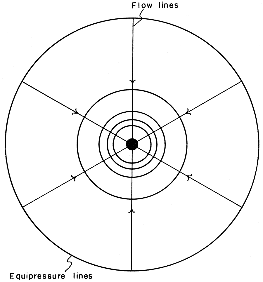
Consider a pumping well in steady state, that is, registering no further drawdown during constant discharge. If Darcy's law is valid, the vertical section of the cone of depression is logarithmic in form. Information obtained from numerous observation wells defines the exact surface of the cone of depression. Figure 3 shows an areal plot of a cone of depression in steady state. No regional gradient is assumed. The outer circle is the boundary of effective radius, the inner concentric circles are lines of equal hydraulic head, and the well is in the center.
Figure 3—Areal plot of cone of depression in steady state.
When the analog plotter is applied to the same situation, the outer boundaries and pumping wells are first painted to scale on the conducting paper. A current is then passed between the electrodes that serve as boundaries. Equipotential lines are readily plotted and give the illusion of being correct. These lines do not coincide with the lines of equal hydraulic head in the pumping well, however. The reason for the discrepancy is the failure of the model to duplicate the geometry of the situation. The current is passed through a paper of constant thickness, whereas the dewatered bed has varying thickness (Fig. 4).
Figure 4—Vertical section showing error in plot caused by failure to account for drawdown in well. Dashed lines are extensions of equipotential and equipressure points.
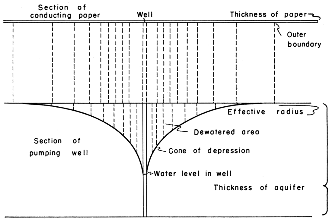
The model depicts a two-dimensional surface, whereas the actual well involves three dimensions. It follows that error in the plot increases with drawdown. In other words, the more the well develops a three-dimensional aspect, the greater will be the error in the two-dimensional plot.
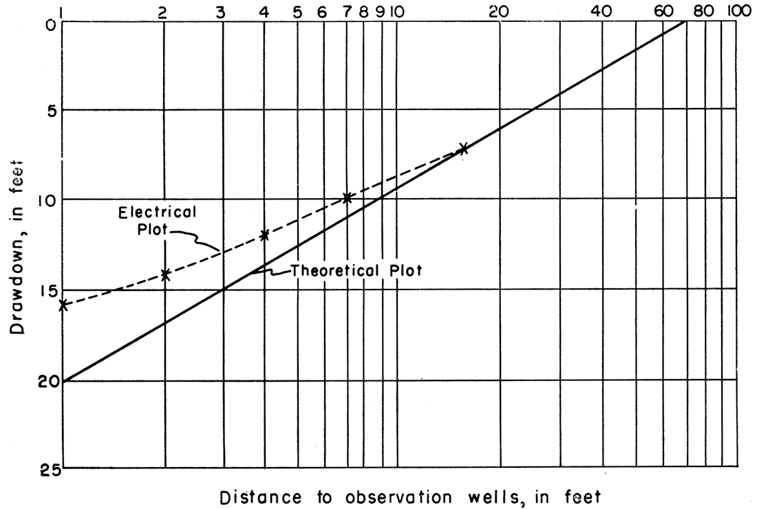
Electrically speaking, the inaccuracy occurs because the electric flow in the conducting sheet varies in only two directions (on the surface of the paper) and is constant in the third direction (the thickness of the paper). For a true analogy, allowance would also have to be made for fluctuations in the third dimension. Figure 5 shows variation between the theoretical logarithmic curve (a straight line) and the curve of the model plot (a curve).
Figure 5—Example of variation between theoretical and electrical plot.
It would seem that this difficulty could be overcome by using a carbon block cut in the same configuration as the well flow system. Exact reproduction of the flow-system geometry on an experimental scale would be a major problem, however. Any deviation from the original system would produce inaccurate results.
Profile plots of steady-state gravity flow.-Another common graphical representation of a flow problem is the profile plot illustrating a vertical section of a well. If the well is pumped in a steady-state condition satisfying the assumptions previously made, a cone of depression develops (Fig. 6).
Figure 6—Block diagram of an ideal flow net system showing equipressure lines and orthogonal flow lines.
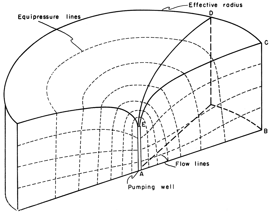
In order to plot a profile section of a radial flow system, a wedge of conductive material must be used instead of the conducting paper, if the analogy is to be retained. That is, the wedge, ABCDEF, of Figure 6 is a proportional and representative sample of the cylindrical flow system.
Because there is more material in the thick base of the wedge, the resistance is lower and consequently the equipotential lines are spaced farther apart. Clearly, the reverse applies at the edge. Carbon wedges have been used on the plotter to obtain substantially correct flow nets (Babbitt and Caldwell, 1948; Wyckoff and Reed, 1935).
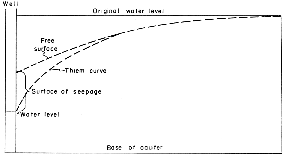
Free surface is defined as the "fluid surface in equilibrium with the atmosphere" (Muskat, 1937, p. 287). Observations reveal that the free surface near a well varies from the Thiem logarithmic curve when the total drawdown is greater than approximately one fifth the thickness of the saturated aquifer (Babbitt and Caldwell, 1948).
The surface of seepage is defined as the surface between the free surface and the actual level of the water in the well. Figure 7 shows the Thiem curve, free surface, surface of seepage, and the water level in a pumping well.
Figure 7—Well profile showing relation of free surface, surface of seepage, and Thiem curve.
The position of the free surface cannot be ascertained directly by use of the analog plotter. There is a trial-and-error method for its location, however, based on the requisite that the pressure differentials have a linear distribution over the surface of the cone of depression. This condition is implicit in the definition of free surface. The following procedure results in defining the free surface.
In Figure 8, the copper boundaries (BC as the anode and AF as the cathode) are scaled to the carbon wedge for a three-dimensional problem or to the conductive sheet for a two-dimensional problem. The potential at D is the same as that at CB. A conducting strip having a resistance greater than that of the electrodes but much less than that of the graphite wedge or paper connects F and D. The potential drop is marked off linearly between F and D. Current is then passed between CB and FA.
Figure 8—Profile plot on electrical model. EC represents the free surface. (Adapted from Wyckoff and Reed, 1935).
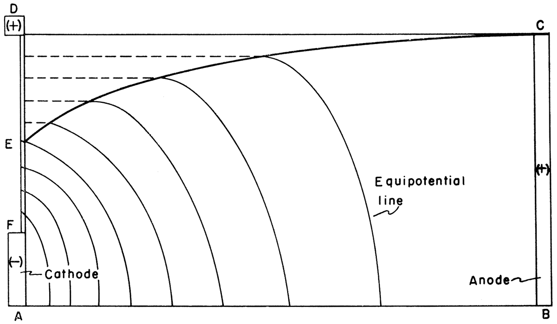
The conducting material is progressively trimmed away from D toward EC, finally forming the trace of EC when the equipotential lines between FA and CB intersect EC at the projections of the points of linear spacing between F and D. The trace of the free surface has now been located, and plotting may proceed.
The analogy between the flow of fluids and electric current does exist, and if the limitations of the analogy are recognized, the plotter can serve some useful purposes.
If the ratio of the drawdown to the total thickness of the aquifer is negligible, an areal plot is sufficiently correct. Single or multiple well data may be plotted if it is remembered that the greatest error develops near the well.
Plotting a single well is a relatively simple affair. The well and the effective boundary are plotted to scale with silver paint on the conductive paper. For the sake of simplicity, resistors can be applied to the electrodes (boundaries) so that drawdowns can be read directly from the potentiometer dial. Current is passed between the electrodes, and equipotential lines are plotted with a probe. A family of circular contours is obtained similar to Figure 3.
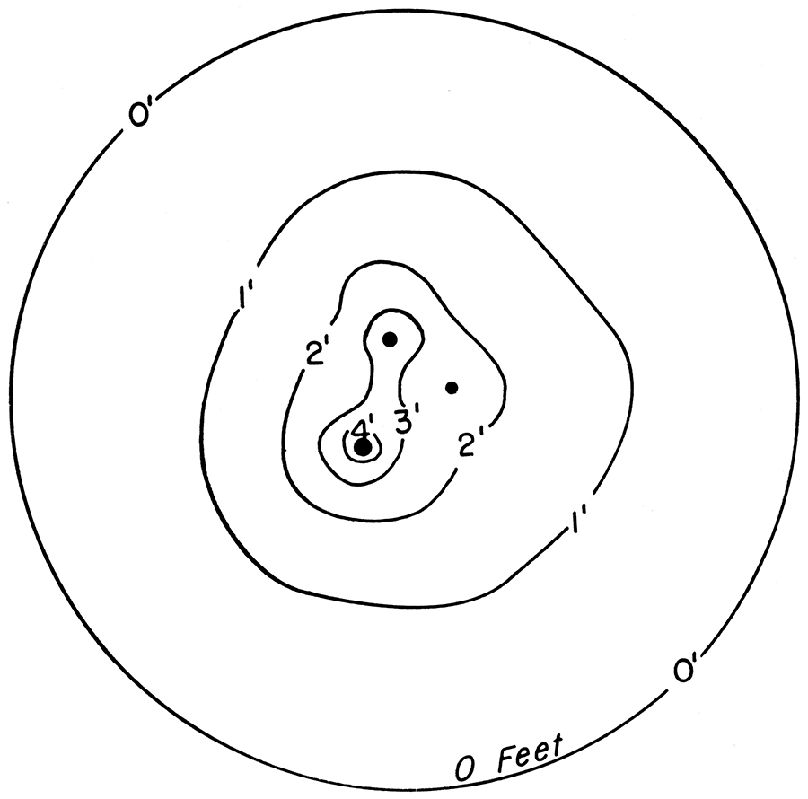
Multiple wells present a more complex problem. Again, the plot only approximates the situation; accuracy is inversely proportional to the relative amount of drawdown. The wells and their effective boundary are painted on the conductive sheet. Resistors can be adjusted so that the potentiometer dial will read the drawdown values for each well even though the values of the wells may differ. When equipotential points are connected, a configuration such as Figure 9 results.
Figure 9—Areal plot of well field showing lines of equal drawdown, in feet.
Accurate plots may be made of situations where only two dimensions vary. If variation in the third dimension can be regarded ail constant or infinite, the plotter may still prove useful. Earthen dams or flows through a straight drainage or irrigation ditch, river, or infiltration gallery are examples of two-dimensional situations in which the plotter may be used advantageously. In analyzing these situations, it still is necessary to locate the free surface in order to draw accurate flow nets.
The conducting-sheet analog field plotter can be applied accurately to ground-water flow problems only when the following conditions exist:
The field plotter cannot be applied accurately to areal plots of three-dimensional, radial, gravity-flow problems, because electric flow has no analog for a variable third dimension in fluid flow. Only an approximation to the true areal plot may be realized. If an aquifer is assumed to have a uniform thickness, a large draw down will produce a greater error than a small drawdown. If a well is assumed to have a constant drawdown, a small effective radius will produce a greater error than a large effective radius.
A profile plot can be made that seems to be accurate if the carbon-impregnated paper is replaced by a carbon wedge to approximate the geometry of the problem.
The conducting-sheet analog field plotter is restricted to problems of a two-dimensional nature. It may be applied to three-dimensional problems only for obtaining approximate solutions.
Babbitt, H. E., and Caldwell, D. H. (1948) The free surface around, and interference between, gravity wells: Illinois Univ. Eng. Exp. Sta. Bull., no. 374, p. 1-58, fig. 1-27.
Botset, H. G. (1945) The electrolytic model and its application to the study of recovery problems: Am. Inst. Min. Met. Eng., Pet. Tech., TP 1945, p. 1-15.
Bruce, W. A. (1943) An electrical device for analyzing oil-reservoir behavior: Am. Inst. Min. Met. Eng., Pet. Tech., TP 1550, p. 1-13.
Jacob, C. E. (1950) Flow of ground water: in Rouse, Hunter, ed., Engineering Hydraulics: John Wiley & Sons, N. Y., p. 321-386.
Lee, B. D. (1947) Potentiometric-model studies of fluid flow in petroleum reservoirs: Am. Inst. Min. Met. Eng., Pet. Tech., TP 2262, p. 1-26.
Liebmann, G. (1950) Solution of partial differential equations with a resistance network analogue: British Jour. Applied Physics, v. 1, p. 92- 103.
Liebmann, G. (1953) Comparison of electric analogues: British Jour. Applied Physics, v. 4, p. 193-200.
Luthin, J. N. (1953) An electrical resistance network solving drainage problems: Soil Science, v. 75, p. 259-274.
Mason, W. J. (1954) Potentiometric-model study of edge-water encroachment: Colorado School of Mines Quarterly, v. 49, no. 3, p. 1-30.
Maxwell, J. C. (1904) A treatise on electricity and magnetism: 3rd ed., Oxford, Clarendon Press, England.
Muskat, Morris (1937) Flow of homogeneous fluids through porous media: McGraw-Hill, N. Y., p. 1-763.
Slichter, C. S. (1899) Theoretical investigation of the motion of ground waters: U. S. Geol. Survey 19th Ann. Rept., pt. 2, p. 295-384.
Taylor, D. W. (1948) Fundamentals of soil mechanics: John Wiley & Son, N. Y., p. 156-204.
Thiem, G. (1906) Hydrologische Methoden, J. M. Gebhardt, Leipzig, p. 1-56.
Wenzel, L. K. (1942) Methods for determining permeability of water-bearing materials: U. S. Geol. Survey Water-Supply Paper 887, p. 1-192.
Wolf, A. (1948) Use of electrical models in study of secondary recovery projects: Oil and Gas Jour., v. 46, no. 50, p. 94-98.
Wyckoff, R. D., and Reed, D. W. (1935) Electrical conduction models for the solution of water seepage problems: Physics, v. 6, p. 395-401.
Kansas Geological Survey
Placed on web Jan. 2, 2019; originally published Aug. 30, 1957.
Comments to webadmin@kgs.ku.edu
The URL for this page is http://www.kgs.ku.edu/Publications/Bulletins/127_2/index.html