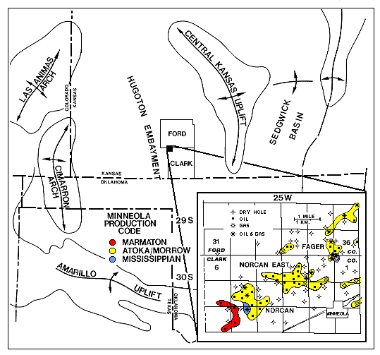
Figure 1. Regional map showing location of the Minneola complex of oil and gas fields in relation to surrounding uplifts and basins (modified from Clark, 1987). Also indicated are productive horizons. The seismic data for this study were acquired over the Norcan and Norcan East fields in T30S, R25W of Clark County.
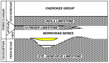	Figure 2. Generalized stratigraphy of the Minneola area (modified from Clark, 1995). Production occurs from marine to fluvial-esturine sandstones surrounded by shales near the top of the Morrowan Series. Although shown as Morrowan, the actual age of these sandstones is debated and may actually be Atokan. Note that the thickest areas of sandstone appear to occur above channels cut into the underlying Mississippian limestone, though they are not limited to occurring above these channels. In addition, not all the channels have productive sandstones above them.
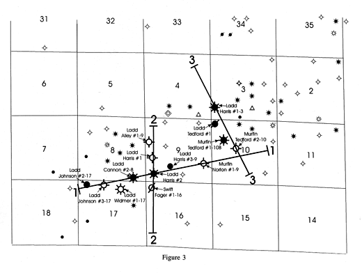	Figure 3. Location map of seismic survey and wells in T30S, R25W. Seismic lines are indicated by dark lines numbered 1 to 3. Major wells used to construct stratigraphic sections and correlate with the seismic data are labeled and have larger well symbols.
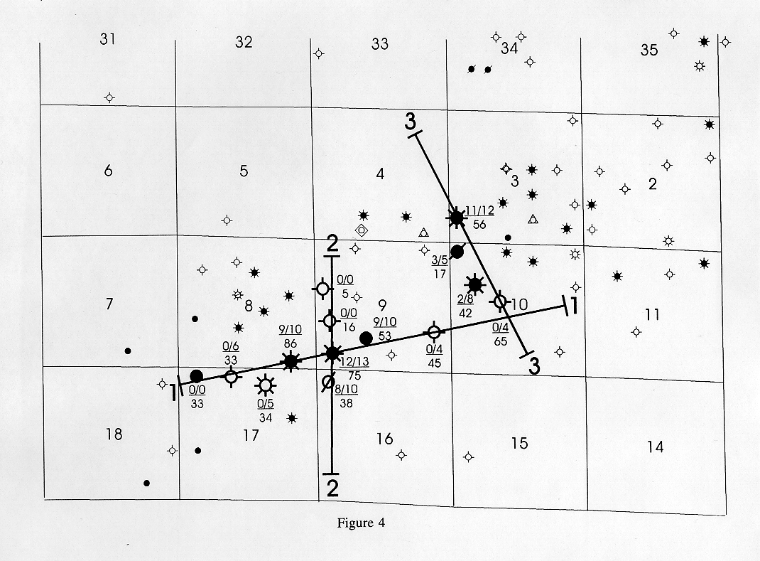	Figure 4. Location map in Figure 3 with net Morrow sand, gross Morrow sand, and Morrow to Mississippian total clastic thickness indicated in major wells. Example is as follows: 0/6 Indicates 0 ft. net sand/6 ft. gross sand 33 33 ft. Morrow-Mississippian
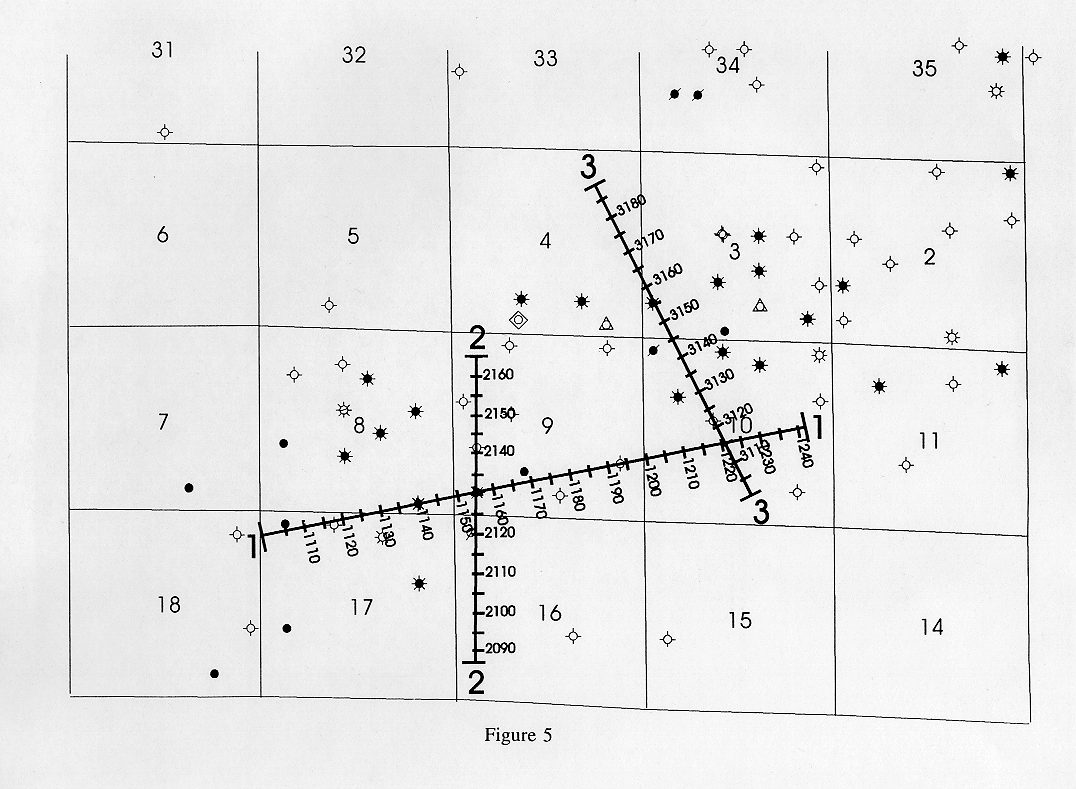	Figure 5. Location map in Figure 3 with receiver station numbers listed for each seismic line. See Appendix A for original shot point locations or contact the Kansas Geological Survey for the SEGP survey locations.
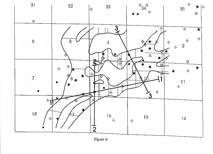	Figure 6. Location map with "channel" locations interpreted from seismic anomalies located on previously acquired seismic data. Solid lines indicate anomaly (channel) boundaries and dotted lines indicate location of seismic lines with anomalies. Most of the seismic data used for this interpretation were acquired with a vibrator source with frequencies after processing below 100 Hz. Seismic lines acquired in this study are also indicated. Note that line 1 runs along a channel while lines 2 and 3 cross one or more channels. Data for map come from Murfin Drilling Company, Wichita, Kansas (written communication).
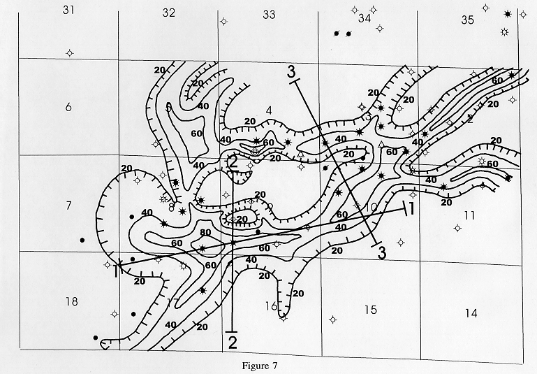	Figure 7. Isopach map of top of Morrow to top of Mississippian indicating thicks associated with interpreted channels. Contour interval is 20 ft. with hatchers on 20 ft. contour pointing towards thicks. Also indicated are seismic lines from present study. Note that line I runs along the axis of one of these thicks while lines 2 and 3 cross one or more thicks.
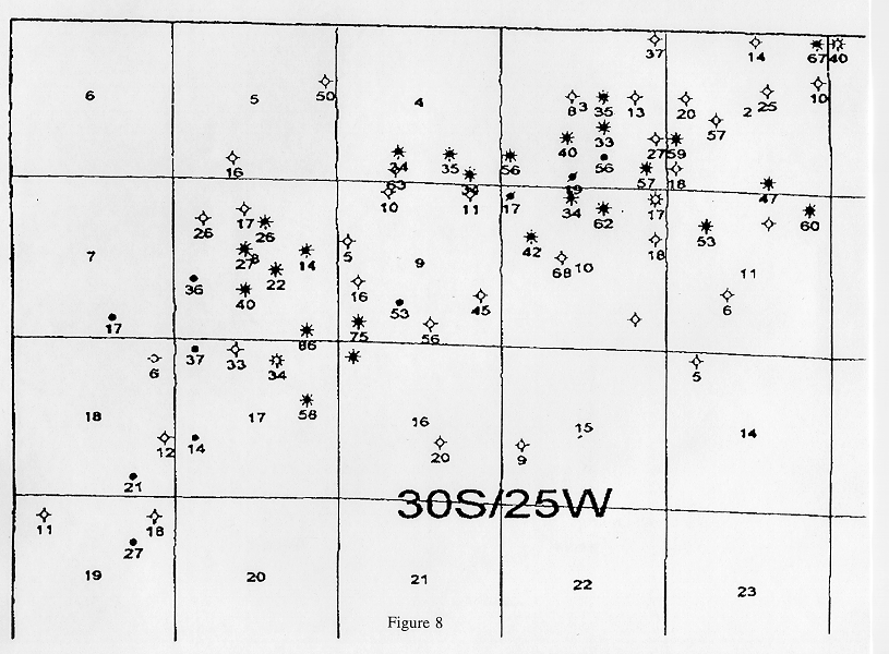	Figure 8. Isopach values used to construct Figure 7 with some values modified along seismic lines based on further investigation of well logs. Map from Murfin Drilling Company, Wichita, Kansas (written communication).
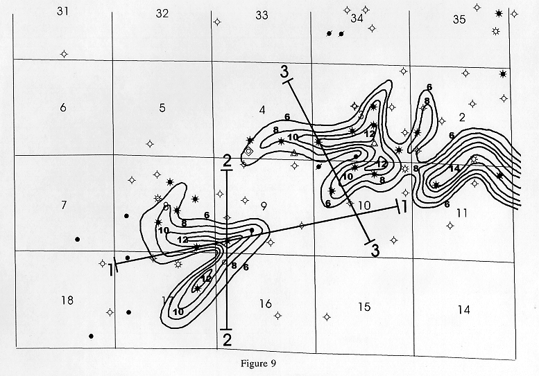	Figure 9. Gross Morrow sand isopach of upper producing sandstone. Contour interval is 2 ft. starting with a minimum thickness of 6 ft. Also indicated are seismic lines from present study. Note that lines cross areas with thick sand as well as no sand.
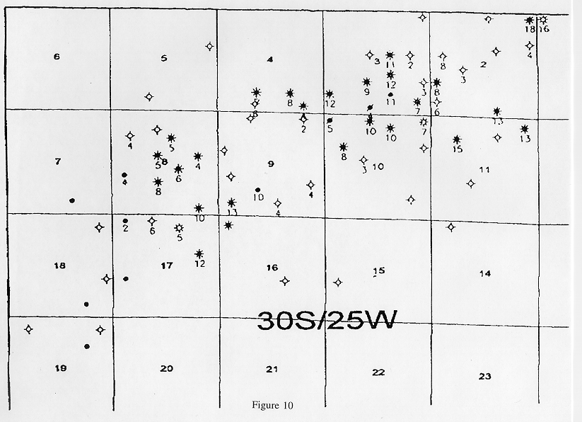	Figure 10. Isopach values used to construct Figure 9 with some values modified along seismic lines based on further investigation of well logs. Map from Murfin Drilling Company, Wichita, Kansas written communication).
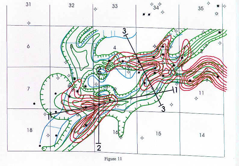	Figure 11. Combined maps of seismic channel anomaly(blue),Morrow to Mississippian isopach (green), and gross sand isopach (red) in Figures 6, 7, and 9, along with seismic lines from present study.
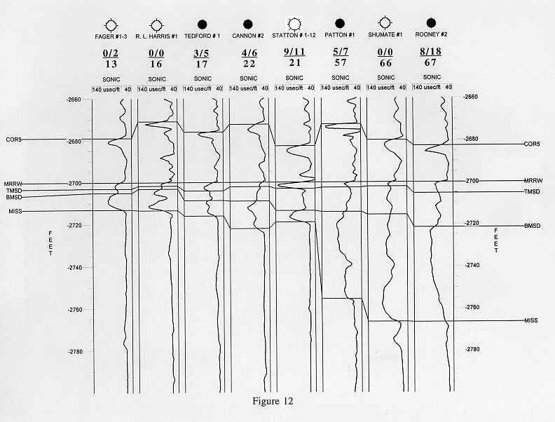	Figure 12. Correlation of sonic logs used for seismic modeling of varying Morrow to Mississippian thickness and sandstone content. Note that the only wells along the seismic lines in this study are the Harris #1 and Tedford #1. This is because they are the only wells along the seismic profiles that contain sonics. See Figure 4 caption for legend of numbers between the well logs and well names. Correlation are MRRW (top of Morrow clastics), TMSD (top of Morrow sandstone), BMSD (base of Morrow sandstone), MISS (top of Mississippian limestone). Correlation is flattened on MRRW. Note that the top and base of sand correlations are carried through wells not containing sand in order to aid in the seism- ic correlation between wells. COR5 is also a marker used to aid correlation between wells. Also note that the density logs for each well were used in the seismic modeling but are not shown here. Locations of wells which are all in T30S-R25W are as follows: Murfin Fager #1-3, SW SE NE sec. 3 Ladd Harris #1, C NW SW sec. 9 Ladd Tedford # 1, NW NW NW sec. 1 0 Ladd Cannon #2, N1/2 NW SE sec. 8 Murfin Statton #1-12, NE NE NW sec. 12 Ladd Patton #1, C SE SE sec. 3 Murfin Shumate #1-13, SW NW NE sec. 13 Ladd Rooney #2, sec. 2
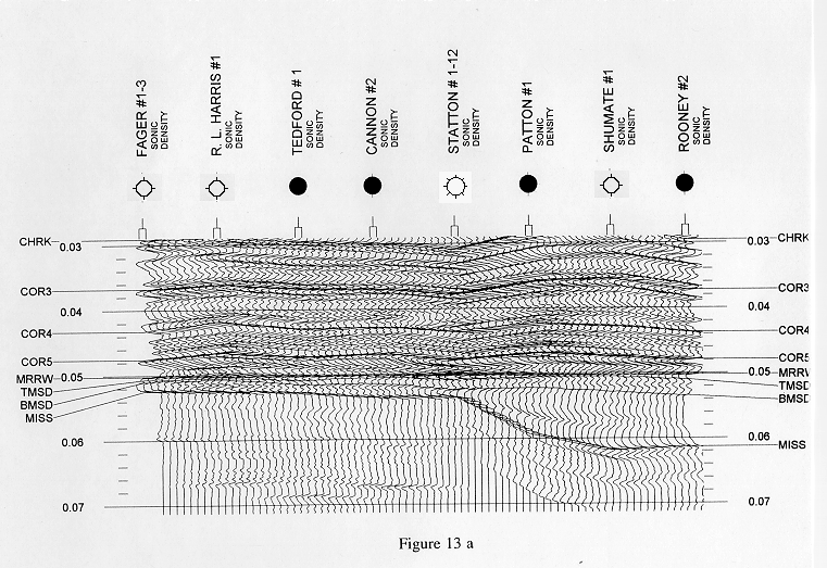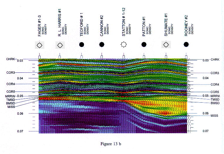
	Figure 13. Acoustic impedance interpolation of sonic and density logs from wells in Figure 12. This interpolated model is used as input for correlation with seismic wavelets to develop the seismic models. Additional correlation markers include the top of the Cherokee (CHRK) and several other unnamed correlation markers. a). Black and white interpolation model with deflections to the right indicating higher impedance and deflections to the left indicating lower impedance. b). Color interpolation model with yellow, orange, and red indicating progressively lower acoustic impedance values and green, blue, and purple indicating progressively higher acoustic impedance values.
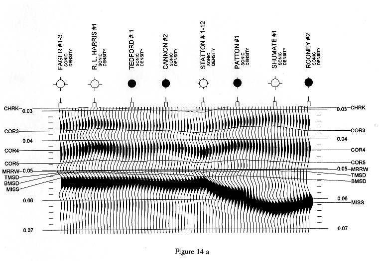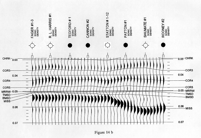
	Figure 14. High-resolution seismic model of varying Morrow-Mississippian thickness and Morrow sandstone thickness. This model was generated by convolving zero phase Ormsby bandpass wavelet (20-30 Hz slope on the low end and 120-180 Hz slope on the high end) with the interpolated acoustic impedance model in Figure 13. a) Every interpolated trace is shown so gradual changes are seen more easily. b) Every other trace is shown so amplitude variations are more visible. c) Red-Blue colors indicate subtle amplitude changes. More intense saturation of red indicates higher amplitude troughs, whereas more intense saturation of blue indicates higher amplitude peaks.
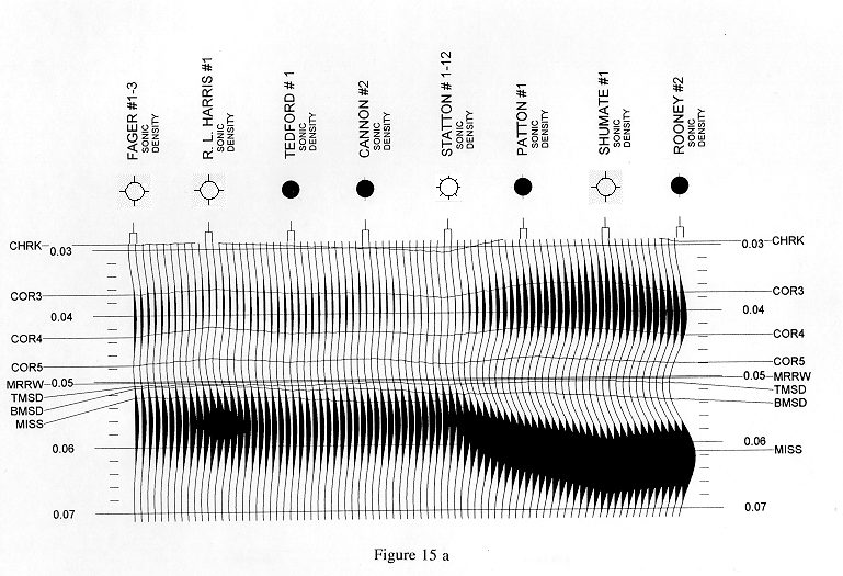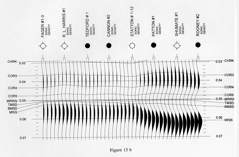
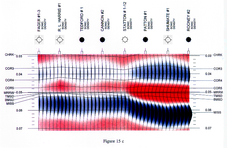
	Figure 15. Low-resolution seismic model of varying Morrow-Mississippian thickness and Morrow sandstone thickness. This model was generated by convolving zero phase Ormsby bandpass wavelet (20-30 Hz slope on the low end and 60-90 Hz slope on the high end) with the interpolated acoustic impedance model in Figure 13. a) Every interpolated trace is shown so gradual changes are seen more easily. b) Every other trace is shown so amplitude variations are more visible. c) Red-Blue colors indicate subtle amplitude changes. More intense saturation of red indicates higher amplitude troughs, whereas more intense saturation of blue indicates higher amplitude peaks.
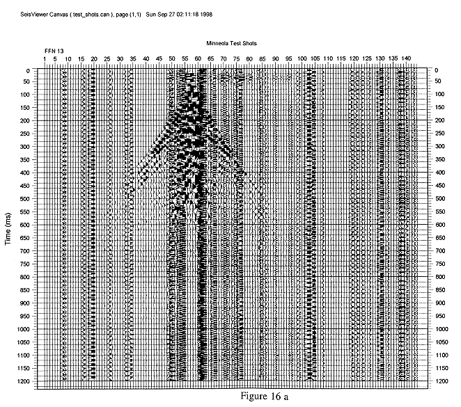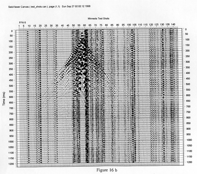
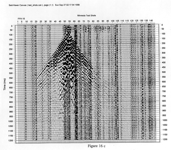
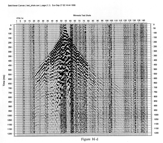
	Figure 16. Selected uncorrected shot gathers from test shots recorded along Line I before acquisition of the three seismic profiles. a) Field File number 13 shot with a 2 lb. Pentalite directed charge at 20 ft. depth with a 20 ft. sand-gravel pack fill of the hole. b) Field File number 6 shot with a 2 lb. Pentalite directed charge at 20 ft. depth with cuttings filling the hole. c) Field File number 15 shot with a 2.5 lb. Seisgel conventional charge at 20 ft del)th with cuttings filling the hole. d) Field File number 14 shot with a 5 lb. Seisgel conventional charge at 20 ft depth with cuttings filling the hole.
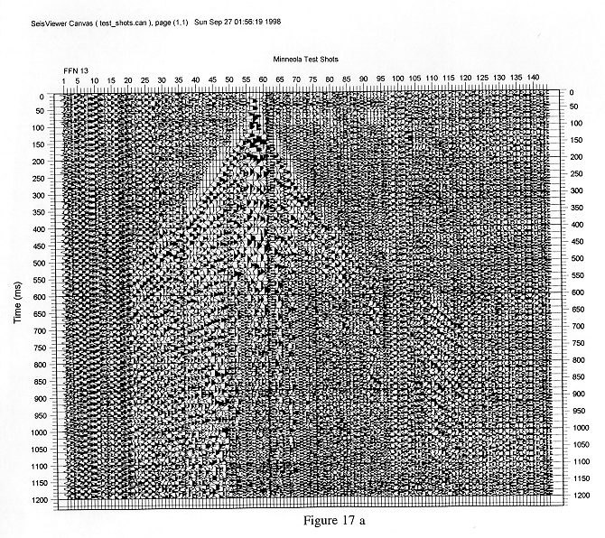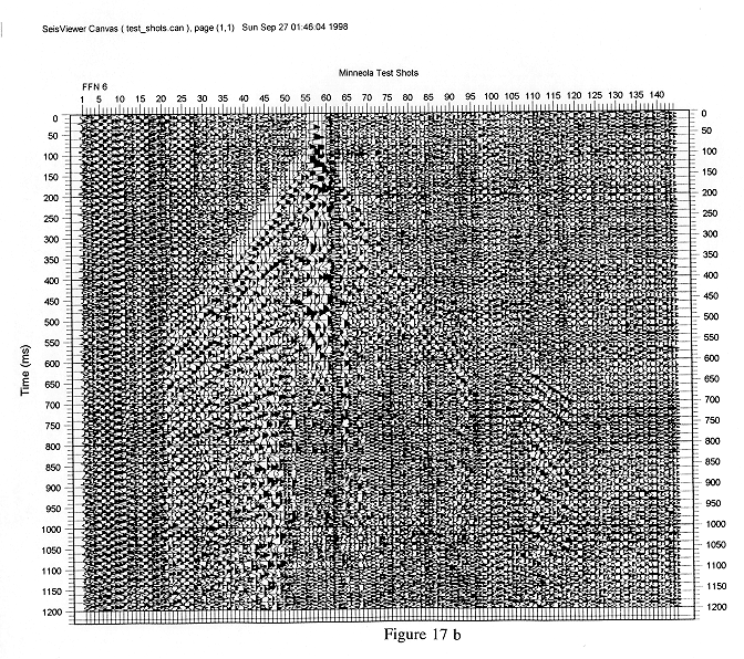
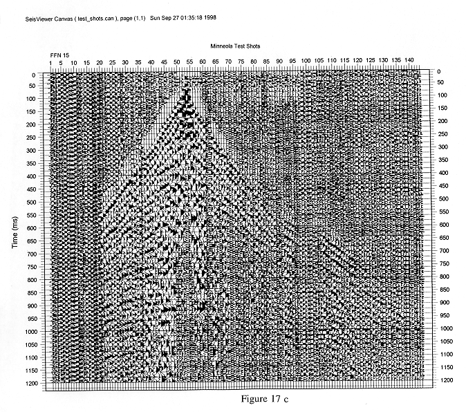
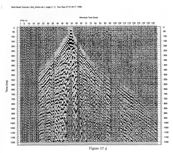
	Figure 17. Selected shot gathers of Figure 16 with AGC applied to enhance reflected events. a) Field File number 13 shot with a 2 lb. Pentalite directed charge at 20 ft. depth with a 20 ft. sand-gravel pack fill of the hole. b) Field File number 6 shot with a 2 lb. Pentalite directed charge at 20 ft. depth with cuttings filling the hole. c) Field File number 15 shot with a 2.5 lb. Seisgel conventional charge at 20 ft depth with cuttings filling the hole. d) Field File number 14 shot with a 5 lb. Seisgel conventional charge at 20 ft depth with cuttings filling the hole.
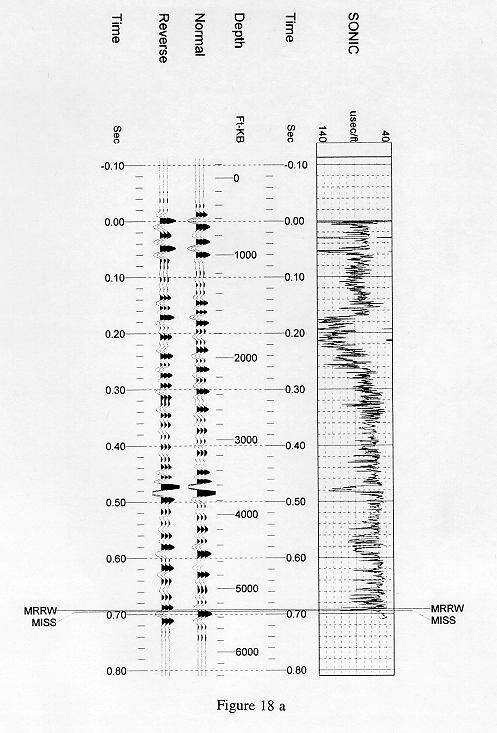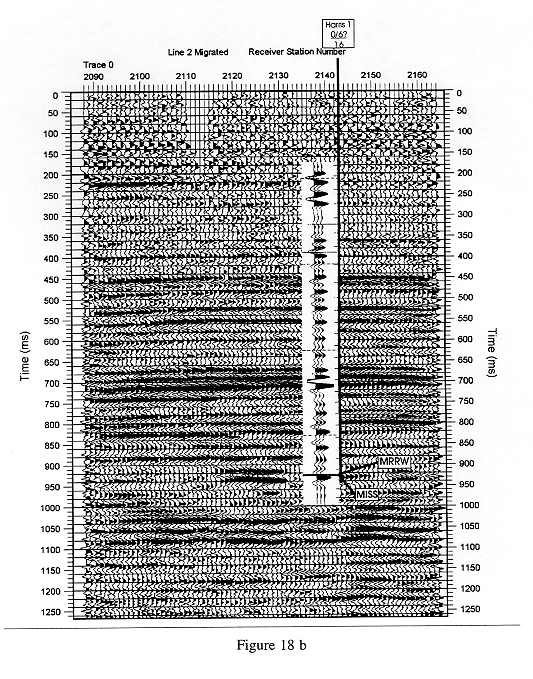
	Figure 18. a) Synthetic seismogram of the Harris #1 well generated with a time varying zero phase Butterworth filter and both the sonic and density logs. The Butterworth filter has the following characteristics: 20 Hz, 36 dB/octave slope - 60 Hz, 72 dB/octave slope down to 500 ms; 20 Hz, 36 dB/octave slope - 50 Hz, 72 dB/octave slope from 500 ms to the bottom. Both negative and positive polarity synthetics are shown with the sonic log. Correlation tops include MRRW (Morrow clastic interval) and MISS (Mississippian limestone). b) Correlation of normal polarity synthetic with Line 2 (migrated section with reverse of field polarity and every other trace displayed). Well location indicated by thick, black vertical line.
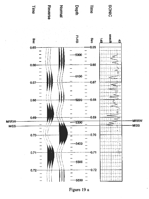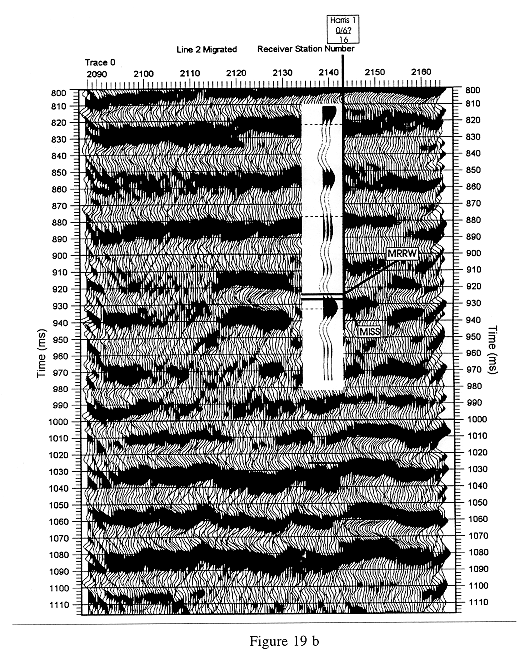
	Figure 19. a) Same as Figure 18a but focused near the Morrow clastic section b) Same as Figure 18b but focused on the Morrow clastic section and with every trace displayed.
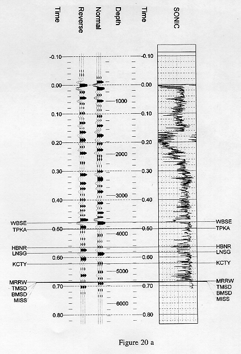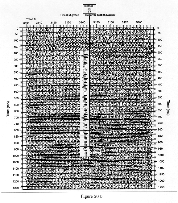
	Figure 20. a) Synthetic seismogram of the Tedford #1 well generated with a time varying zero phase Butterworth filter and both the sonic and density logs. The Butterworth filter has the following characteristics: 20 Hz, 36 dB/octave slope - 60 Hz, 72 dB/octave slope down to 520 ms; 20 Hz, 36 dB/octave slope - 50 Hz, 72 dB/octave slope from 520 ms to the bottom. Both negative and positive polarity synthetics are shown with the sonic log. Correlation tops include ) WBSE (Wabaunsee Group), TPKA (Topeka Limestone), HBNR (Heebner Shale), LNSG (Lansing Group), KCTY (Kansas City Group), MRRW (top of Morrow clastic interval) and MISS (top of Mississippian limestone). b) Correlation of normal polarity synthetic with Line 3 (migrated section with reverse of field polarity and every other trace displayed). Well location indicated by thick, black vertical line.
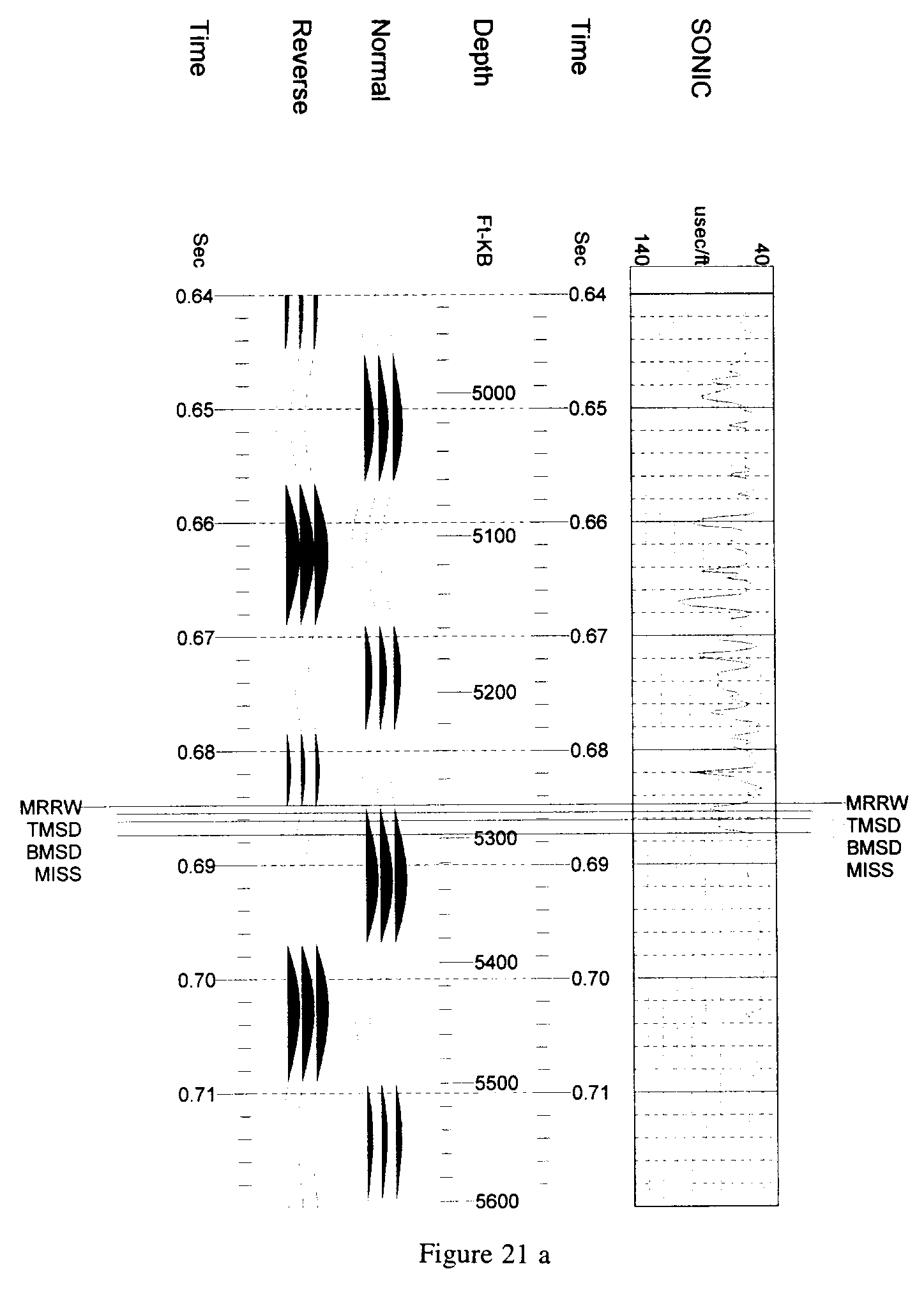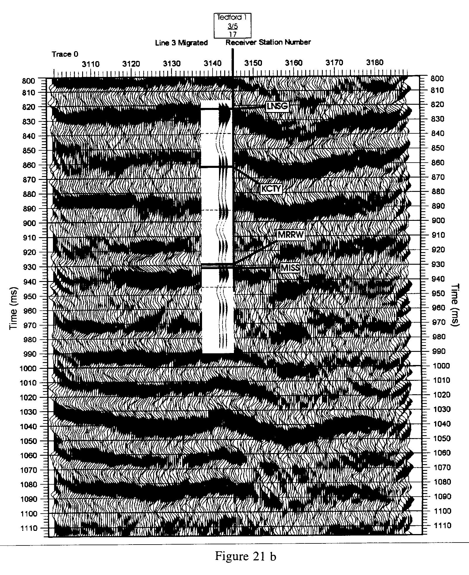
	Figure 21. a) Same as Figure 20a but focused near the Morrow clastic section b) Same as Figure 20b but focused on the Morrow clastic section and with every trace displayed.
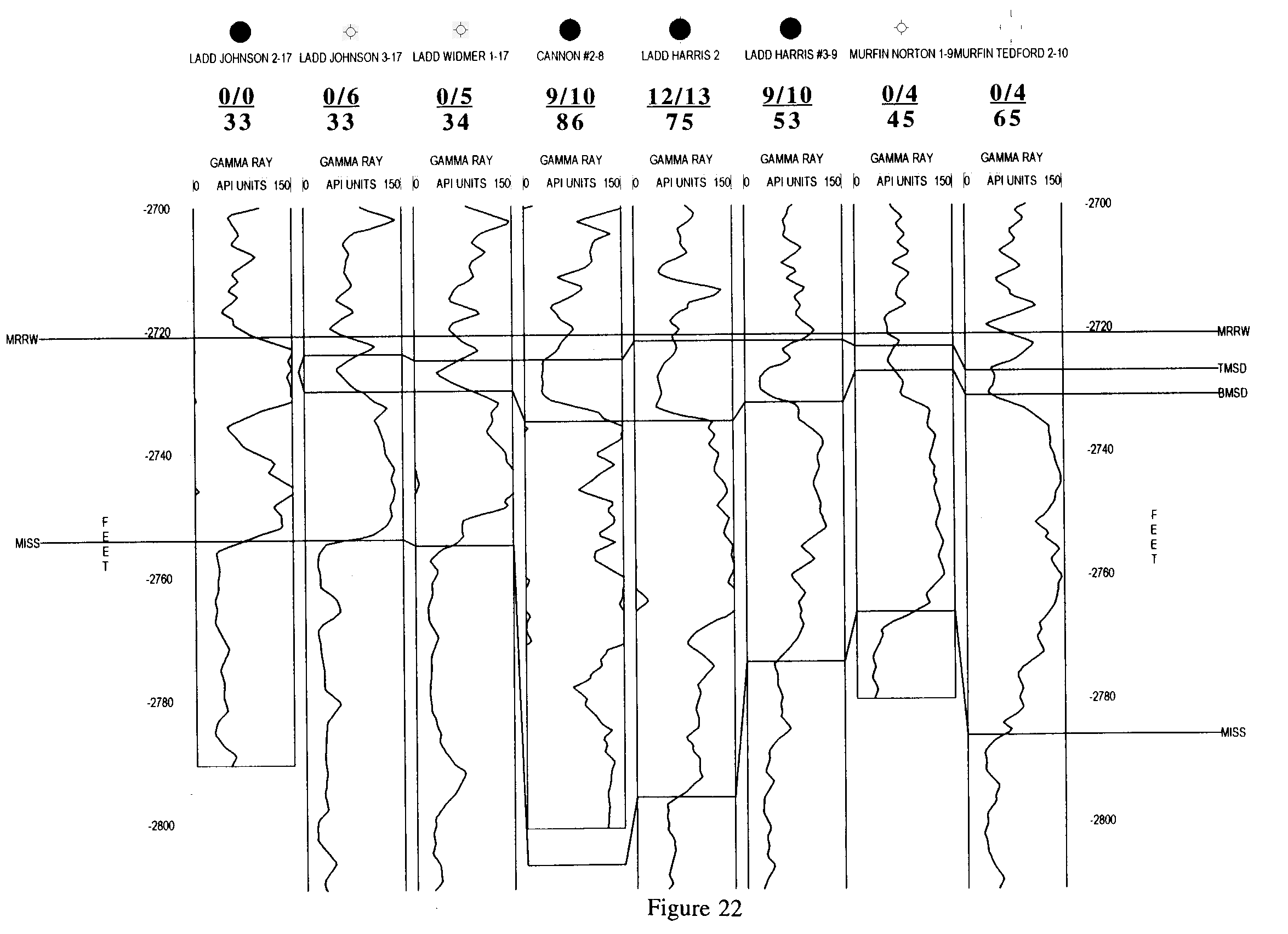	Figure 22. Correlation of gamma ray logs along Line I to show varying total Morrow clastic interval thickness and the gross sandstone thickness near the top of the Morrow clastic section. See Figure 4 caption for legend of numbers between the well logs and well names. Correlations are MRRW (top of Morrow clastics), TMSD (top of Morrow sandstone), BMSD (base of Morrow sandstone).
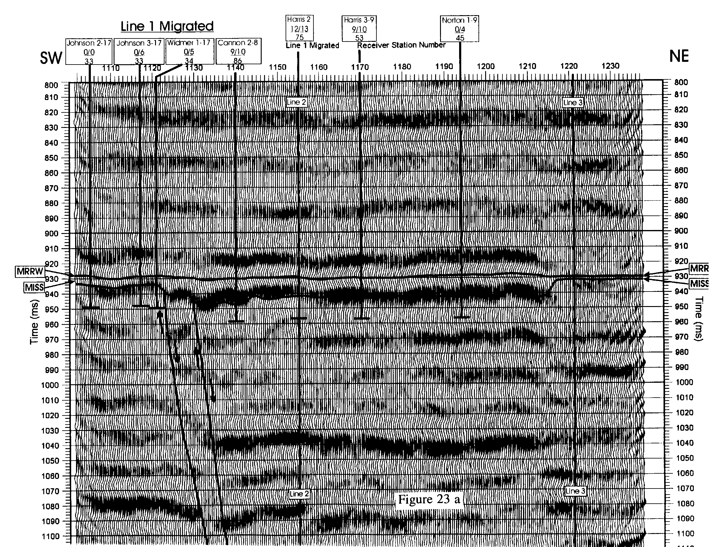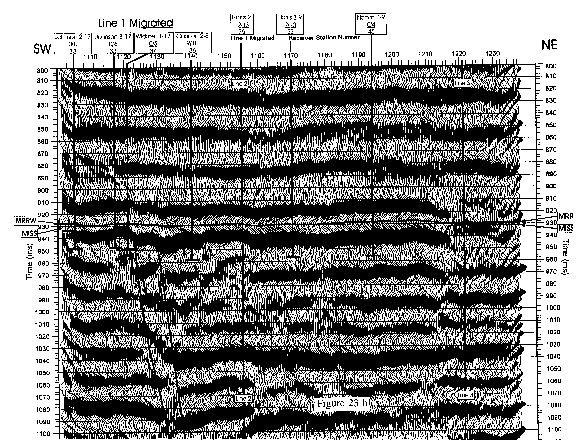
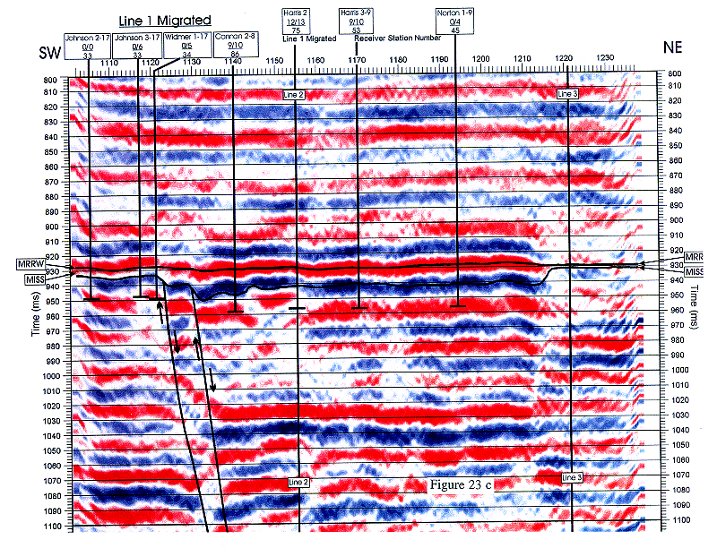
	Figure 23. Interpretation of the migrated version of Line 1 centered on the Morrow clastic interval. Shown are the top of the Morrow clastic interval (MRRW) and top of Mississippian limestone (MISS), well ties (thick black vertical lines indicate location and probable total depth of wells), net sand thickness, gross sand thickness, and thickness of the total Morrow clastic section in the wells (see Figure 4 for explanation of number code), ties with Lines 2 and 3 (vertical black lines through entire section), and faults (thick black lines with arrows showing relative movement across fault. Receiver station numbers along top of section correspond to those in Figure 5. a) Section with a -10 dB/octave gain applied before display to help amplitude of peaks stand out. b) Section with no gain to allow amplitude of troughs to stand out. c) Red (troughs) - blue (peaks) section to aid in amplitude interpretation. Higher intensity saturation of reds and blues indicate higher amplitudes.
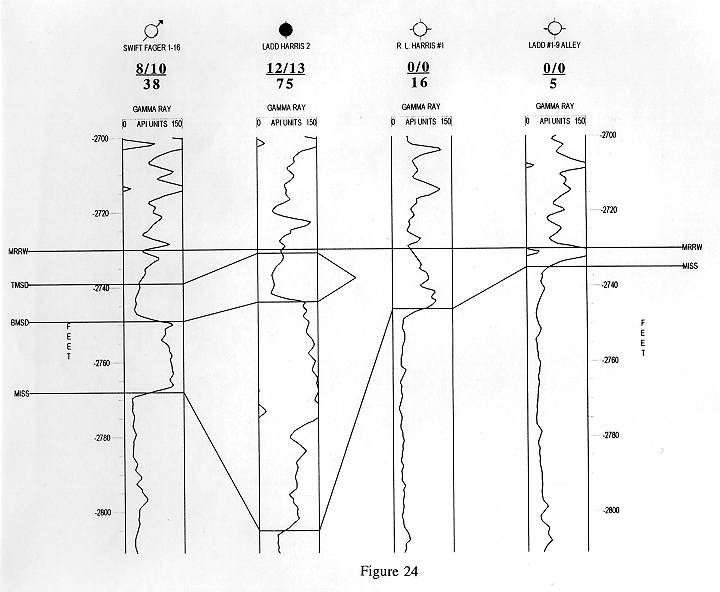	Figure 24. Correlation of gamma ray logs along Line 2 to show varying total Morrow clastic interval thicknesses and the gross sandstone thickness near the top of the Morrow clastic section. See Figure 4 caption for legend of numbers between the well logs and well names and Figure 22 for correlation abbreviations.
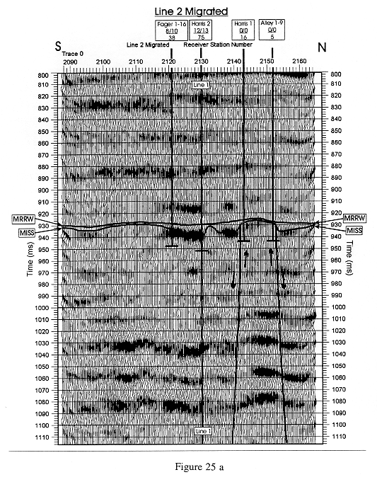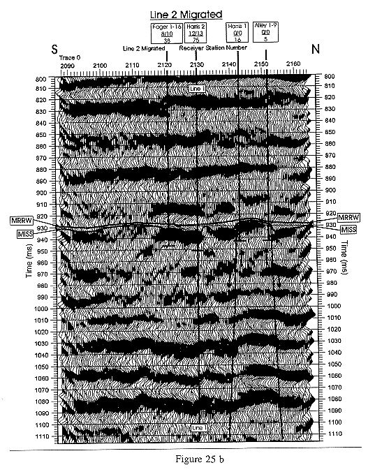
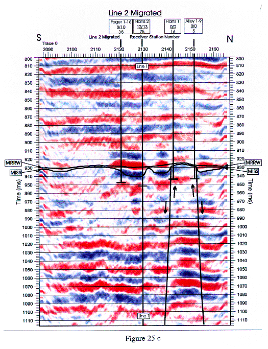
	Figure 25. Interpretation of the migrated version of Line 2 centered on the Morrow clastic interval. Shown are the top of the Morrow clastic interval (MRRW) and top of Mississippian limestone (MISS), well ties (thick black vertical lines indicate location and probable total depth of wells), net sand thickness, gross sand thickness, and thickness of the total Morrow clastic section in the wells (see Figure 4 for explanation of number code), tie with Line 1 (vertical black line through entire section), and faults (thick black lines with arrows showing relative movement across fault. a) Section with a -10 dB/octave gain applied before display to help amplitude of peaks stand out. b) Section with no gain to allow amplitude of troughs to stand out. c) Red (troughs) - blue (peaks) section to aid in amplitude interpretation. Higher intensity saturation of reds and blues indicate higher amplitudes.
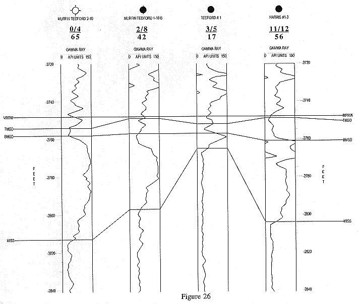	Figure 26. Correlation of gamma ray logs along Line 3 to show varying total Morrow clastic interval thickness and the gross sandstone thickness near the top of the Morrow clastic section. See Figure 4 caption for legend of numbers between the well logs and well names and Figure 22 for correlation abbreviations.
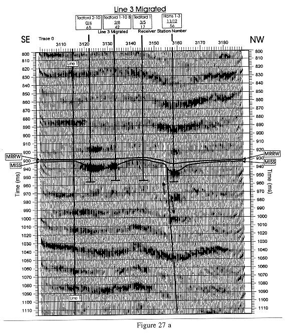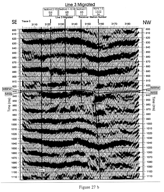
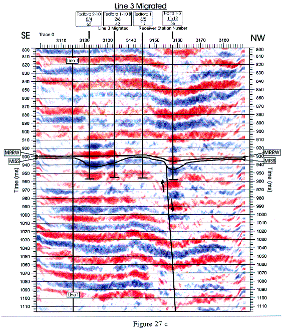
	Figure 27. Interpretation of the migrated version of Line 3 centered on the Morrow clastic interval. Shown are the top of the Morrow clastic interval (MRRW) and top of Mississippian limestone (MISS), well ties (thick black vertical lines indicate location and probable total depth of wells), net sand thickness, gross sand thickness, and thickness of the total Morrow clastic section in the wells (see Figure 4 for explanation of number code), tie with Line 1 (vertical black line through entire section), and faults (thick black lines with arrows showing relative movement across fault. a) Section with a - 1 0 dB/octave gain applied before display to help amplitude of peaks stand out. b) Section with no gain to allow amplitude of troughs to stand out. c) Red (troughs) - blue (peaks) section to aid in amplitude interpretation. Higher intensity saturation of reds and blues indicate higher amplitudes.
	Figure 28. Figure 6 with channel (seismic anomaly) boundaries and channel anomalies on seismic lines indicated by dashed lines. Solid lines modify the channel boundaries interpreted from previous seismic data by incorporating results from current seismic experiment. Seismic lines of current experiment with receiver station locations are also shown.