Kansas Geological Survey, Open-file Report 96-36
by
Alex Martinez (Kansas Geological Survey),
D. Scott Beaty (Kansas Geological Survey),
Howard R. Feldman (Exxon Research and Production Corporation), and
Joseph M. Kruger (Kansas Geological Survey)
KGS Open File Report 96-36
September 1996
This paper is an adaptation of a poster presented at the 1996 annual AAPG meeting in San Diego.
Small-scale lateral variations in sandstone permeability and porosity can have dramatic implications for oil and gas field development and productivity. Unfortunately, these variations occur at scales much smaller than typical well spacing, such that one must turn to outcrop analogs in order to predict the architecture of small-scale stratigraphic complexities.
The Tonganoxie Sandstone (Upper Pennsylvanian) is thought to be an analog for some Upper Morrow incised valley-fill sandstone reservoirs, and it is productive in at least one location. High-frequency (500 MHz) ground-penetrating radar (GPR) data were used to obtain decimeter-scale resolution from the surface to a maximum depth of 5 m at a study site over the Tonganoxie Sandstone in northeast Kansas. The primary study; data are a grid of 2D profiles spaced 1.5 m apart over a 30.5 m x 30.5 m area. Both individual foresets and bedset bounding surfaces were successfully imaged. Bounding surfaces are potential zones of reduced permeability and may result in reservoir compartmentalization. GPR data were processed using conventional seismic software and interpreted on a workstation to map 3D geometries of bounding surfaces.
Outcrop photomosiacs reveal that tabular planar crossbed sets generally thin upwards from 1.0 m thick at the base of the outcrop to 0.3 m thick near the top, probably reflecting an individual channel fill. GPR results reveal that shapes of sandstone bodies are highly variable, with their long axis either parallel to paleoflow direction or normal to it. At least one sandstone bedset is greater than 30.5 m long. Integration of minipermeameter and GPR data reveal that surfaces of low permeability can be mapped through GPR methods.
The three-dimensional geometries, erosional surfaces, and bedding features of fluvial depositional systems have conventionally been inferred from two-dimensional outcrop and core data. However, outcrops and cores provide limited information, resulting in some ambiguity as to true three-dimensional shapes. This approach may be adequate for the study of very simple features, but does not provide sufficient information for accurate three-dimensional characterization of complex features found in interwell regions.
This paper is the result of a pilot study by the Kansas Geological Survey to determine the feasibility of using high-frequency ground-penetrating radar (GPR) methods to image detailed stratigraphic features within sandstone bodies. A preliminary profile of high-frequency (500 MHz) GPR data was obtained behind an outcrop at a study site located in northeastern Kansas (Figure 1). The results were so promising that a closely spaced grid of data were gathered in hopes of mapping stratigraphic features in three dimensions. In addition, four 1.8-3.1 m (6-10 ft) vertical profiles and one 43.8 m (144 ft) lateral profile of minipermeameter data were gathered from the outcrop face and correlated with the GPR data.
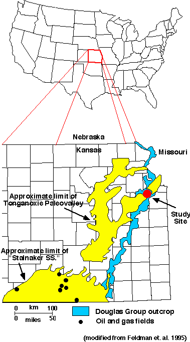
Figure 1. Map showing the location and extent of the Tonganoxie paleovaley. Oil and gas fields in marine sandstone to the south of the site are also shown. The GPR study site is indicated by a star.
The results of the study reveal that high-frequency GPR methods are capable of imaging the subsurface to a maximum depth of approximately 4 m with decimeter-scale resolution. Major bounding surface, such as channel edges, and internal bedding features, such as crossbedding, are readily visible on the GPR data and can be mapped in three dimensions. Also, surfaces of low permeability found using a minipermeameter along the outcrop can be correlated with surfaces imaged via GPR.
The study site is in Wyandotte County, Kansas, over the eastern edge of the Tonganoxie Sandstone Member of the Stranger Formation (Upper Pennsylvanian), a NE-SW trending, incised paleovalley fill located in northeastern Kansas (Figures 1 and 2). It is of economic importance as an aquifer (O'Conner, 1960), and as an analog for hydrocarbon reservoirs (Winchell, 1957).
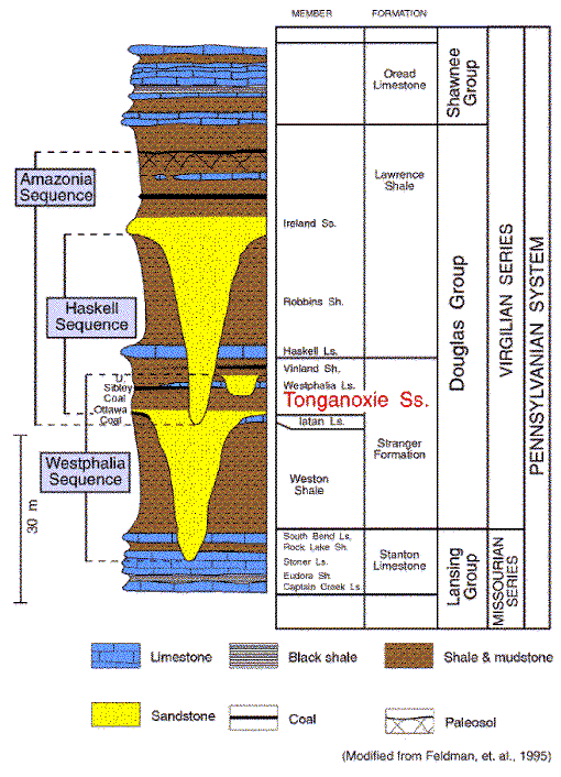
Figure 2. Schematic stratigraphic column of the Tonganoxie Sandstone Member and adjacent units.
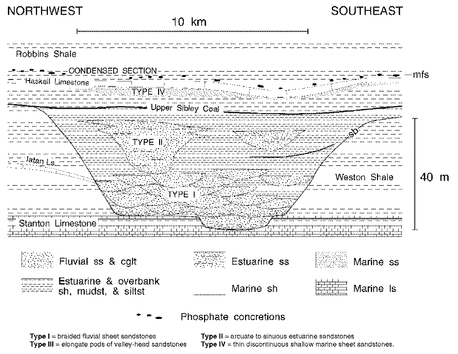
The overall geometry of the paleovalley and its general internal stratigraphy have been studied by conventional methods (e.g., core and outcrop information) (Feldman et. al., 1995; Gibling et. al., 1993). These studies have divided the Tonganoxie Sandstone into four distinct architectural types: (1) braided fluvial sheet sandstones, (2) arcuate to sinuous estuarine sandstones, (3) elongate pods of valley-head sheet sandstones, and (4) thin discontinuous shallow marine sheet sandstones (Figure 3; Feldman et. al., 1995). At the GPR study site, sandstone was deposited as (Type One) braided fluvial sheet sandstone. The meso-scale geology at this site is very complex due to multiple channel cuts during deposition. The paleocurrent direction is east, possibly due to an erosional remnant deflecting the current.
Figure 3. Schematic cross-section of the Tonganoxie paleovalley in the study area (Feldman et. al., 1995). The GPR study site is located in the Type I sandstones.
Ground-penetrating radar (GPR) is a high-resolution near-surface geophysical technique using antennas to send electromagnetic pulses into the ground in order to image the subsurface via returned reflection energy. Similar to seismic reflections, where reflections are caused by boundaries associated with acoustical impedance contrasts, GPR reflections are caused by the electromagnetic waves encountering media of different electrical properties--namely boundaries consisting of a contrast in the dielectric constant of the material above and below the boundary (Davis and Annan, 1989). GPR methods are limited to the very-near surface (usually less than 10 m) due to the high attenuation of the electromagnetic waves through dielectric materials.
GPR profiles have a similar appearance to seismic profiles, and usually are represented as common depth point (CDP) data, with amplitude variations representing differences in reflection strength. A monostatic antenna was used for this study, meaning the same antenna was both the source and the receiver (zero offset data). As with seismic data, vertical scales are in time (or depth if the data have been depth migrated), while lateral scales are in distance. However, the scales differ by several orders of magnitude; GPR records have time lengths measured in nanoseconds (1 x 10⁻⁹ s), compared to milliseconds (1 x 10⁻³ s) in seismic records. Also, the lateral distances between CDPs in GPR profiles are usually much smaller than seismic profiles. The average horizontal (cdp) spacing for this study was 3 cm.
One 229 m (750 ft) long GPR profile, and one 30.5 m x 30.5 m grid of GPR profiles with 1.5 m (5 ft) grid spacings were obtained at the study site (Figure 5). The profiles were flagged at 1.5 m intervals, and relative elevation information was obtained every station along the data grid, and at every fifth station along the individual profile behind the outcrop (Figure 6). A photomosaic of the outcrop was made in order to directly tie the GPR data to the outcrop (Figures 7-10).
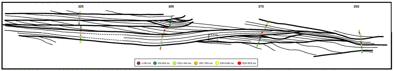
Figure 5. Map of the study site showing the locations of the outcrop, the GPR profiles, and the minipermeameter profiles.
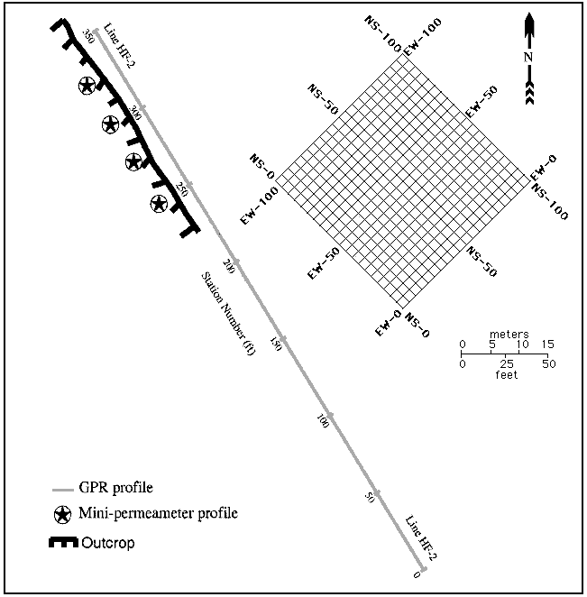
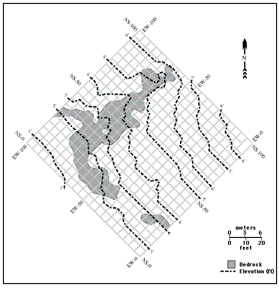
Figure 6. Relative elevation map of the GPR data grid. The location of the exposed bedrock is important for elevation corrections due to the velocity pull-down effect of the soil.
The GPR data were gathered using a GSSI SIR System-8 unit with a 500 MHz dominant frequency monostatic antenna. Use of a monostatic antenna allowed rapid data acquisition, but precluded measurement of any velocity information. A scan length of 80 ns was recorded at a rate of 12.8 scans/s as the antenna was pulled along the line. A pulse was added to the data whenever a flag was passed along the profile to provide lateral control.
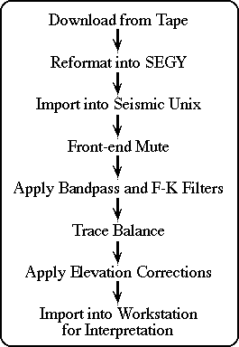
The data were downloaded from a tape unit, converted into SEGY format, and imported into Seismic Unix for data processing, where they were treated as stacked seismic data (Figure 4). The data were static shifted using the relative elevation information and a constant velocity of 0.15 m/ns in order to better represent the true subsurface geometries. Finally the data were imported into a workstation-based seismic-interpretation software package.
Figure 4. Generalized GPR data processing flow chart for this project.
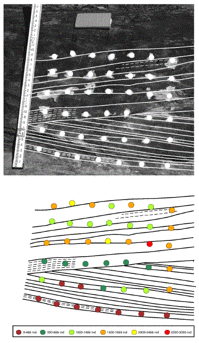
A portable field permeameter (minipermeameter) was used to measure gas permeability values along the outcrop. In order to analyze variations in permeability values, four vertical profiles spaced 7.6 m (25 ft) were established (Figures 8 and 9). For each profile, permeability measurements were made at a vertical spacing of 15 cm (0.5 ft). Permeability was also analyzed in a closely spaced 61 cm x 54 cm (2 ft x 1.75 ft) grid (Figure 10).
Figure 7. Ground-penetrating radar profile gathered approximately 3-5 m behind the outcrop face. This profile was correlated with outcrop information shown in Figures 8 and 9. Interpretations of the major bounding surfaces imaged by GPR are shown by white lines.
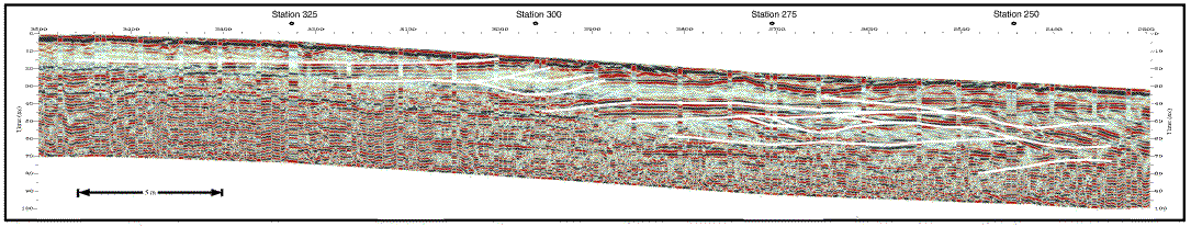
Figure 8. Photomosaic of a portion of the study site outcrop with major bounding surfaces highlighted. Heavier line weights indicate surfaces of erosional truncation, and lighter line weights indicate bedding planes. The outcrop is composed primarily of trough-crossbedded sandstone.
Figure 9. Outcrop schematic showing the locations of bounding surfaces in relation to color-coded minipermeameter data profiles. As expected, bounding surfaces are areas of low permeability. These bounding surfaces were imaged by the GPR profile (Figure 7), meaning that GPR can be used in locating low permeabiloty surfaces.
As shown in Figure 9, permeability profiles indicate that values are highly variable, ranging from 100 to 2500 millidarcies (md), but are relatively consistent within individual channels. The closely spaced permeability grid in Figure 10 demonstrates that mud-draped micaceous surfaces on lamina sets are responsible for lower permeability values. Clay mineral and mica content generally increases near the top of the trough-fills and some troughs contain abundant clay rip-up clasts near their erosional base. Clay- and mica-rich sandstone troughs are common near the top of the outcrop and have relatively low gas permeability values but high electrical permittivity values (resulting in strong GPR reflections). Additional research is necessary in order to investigate the relationships between electrical permittivity and gas permeability. If a clear-cut relationship exists between the two values it may be possible to construct a three-dimensional depiction of gas permeability in gridded areas based upon permittivity.
Figure 10. A closely-spaced grid of minipermeameter measurements (10 cm apart) was gathered at the outcrop face to determine small-scale variations in permeability values. Bounding surfaces are shown in relation to minipermeameter data. These surfaces typically have lower permeability values.
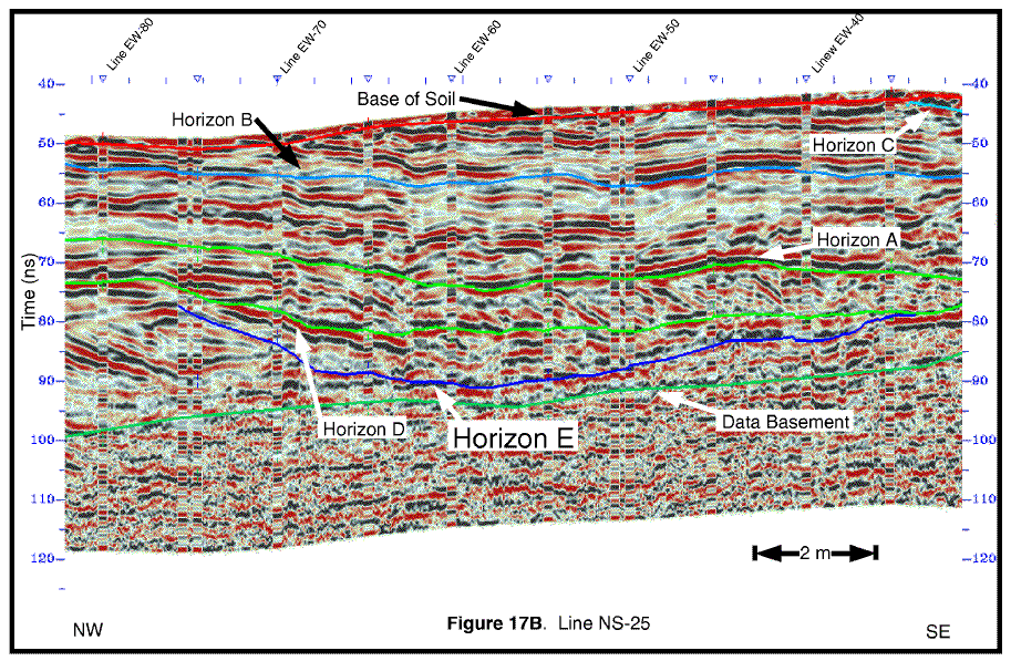
Interpretations of gridded GPR data were made using a computer workstation. The data were divided into small- and large-scale groupings of similar bedding type. Where possible, large-scale groupings were further subdivided into small-scale groupings. For this pilot study only the most prominent horizons were selected for interpretation. This method yielded five major horizons: (1) data basement, (2) Horizon A, the base of a large channel fill, (3) Horizon B, the base of a convoluted planar bedded interval, (4) Horizon C, the base of a planar bedded interval, and (5) the base of the soil. The interval between the data basement and Horizon A was subdivided by Horizons D and E, the bases of two small channel-fills. The interval between Horizons A and B contains several different bedsets with complex three-dimensional geometries. As most of these bedsets are extremely small in scale, this interval has not been fully subdivided yet.
As seen by the variable time-depth of the interpreted data basement, data quality varied across the gridded area. The highest quality data were gathered from exposed bedrock surfaces (see Figure 6), and the poorest quality data were gathered from areas of relatively thick soil cover (0.5 - 1.0 m), such as along the northern edge of the data grid. The amount of soil cover affected data interpretation by causing a velocity pull-down effect (i.e., the velocity of the soil is slow relative to the velocity of the sandstone). In order to negate the effects of velocity pull-downs, deeper horizons such as A, D, and E were interpreted from cross sections which utilized the relatively flat bases of either horizon B or C as a datum.
Isochron maps were used to analyze the general thickness of each interval, but it was not always possible to extend these maps throughout the limits of the gridded area. Where the tops of the intervals are truncated by the modern erosional surface it is not known how much material was removed. Because of this, the interval from Horizon B to Horizon C is shown in map view as both an isochron map (Figure 14A), and an areal extent map (Figure 14B). Because of the effects of soil velocities on the vertical distribution of data, structural maps of the various horizons were not deemed a valid method of displaying the data.
Figure 14A. Isochron map of the interval from Horizon B to Horizon C. This interval consists of convoluted, originally planar beds. Horizon B is the erosional base of this interval.
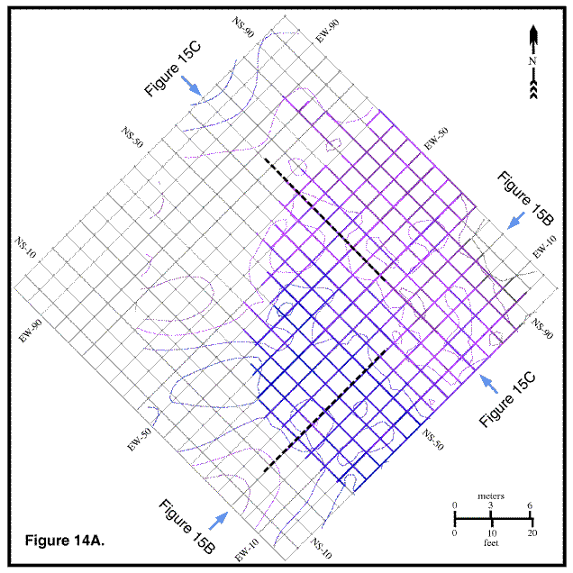
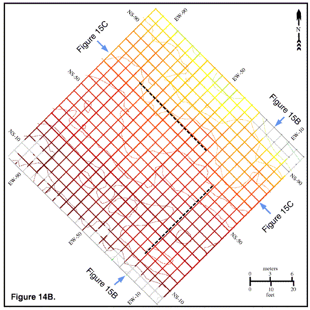
Figure 14B. Map showing the extent of Horizon B. This horizon, the base of a convoluted planar bedding interval, has contact with the modern erosional surface over some of its area. As can be seen on the time-depth map below, the surface is relatively planar.
The erosional base of a large channel-fill, this horizon extends across the entire data grid. The data grid is only over one flank of the paleochannel, which was approximately 45-60 m in width. The paleochannel trends in a NW-SE direction, and has an incised feature near the center of the data grid. The A-B interval (Figure 13) contains several bedsets with different paleoflow directions.
Figure 13A. Isochron map of the interval from Horizon A to Horizon B. Horizon A is a major bounding surface extending across the entire data grid. It is interpreted as the side of a paleochannel, and truncates several bedsets on the southern edge. It is similar to the large channel seen on the outcrop photomosaic (Figures 7-9). The top of this interval, Horizon B, is an erosional contact with the base of a convoluted planar-bedded interval.
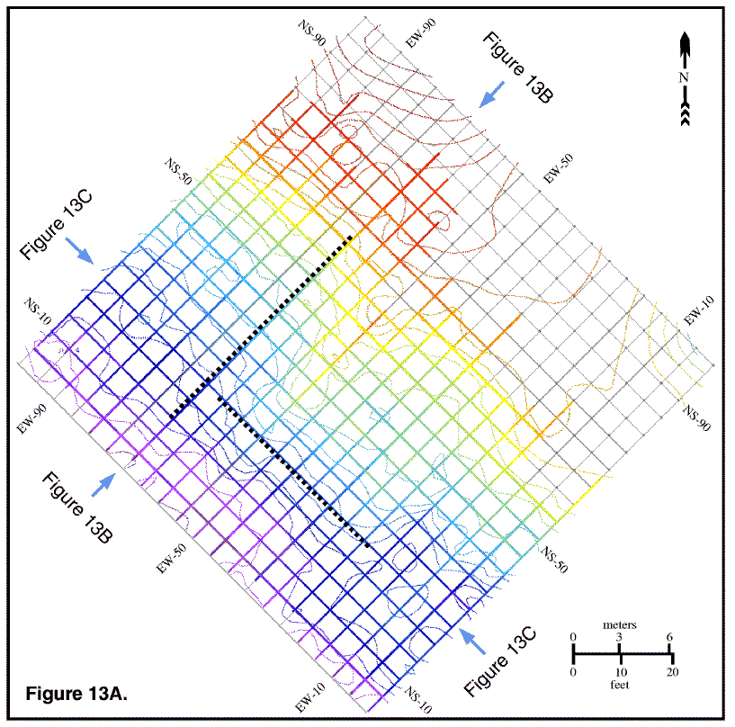
Figure 13B. A portion of the GPR profile from Line EW-70. The diffractions within the A to B interval along the NE side of the line are interpreted to result from ironstone nodules.
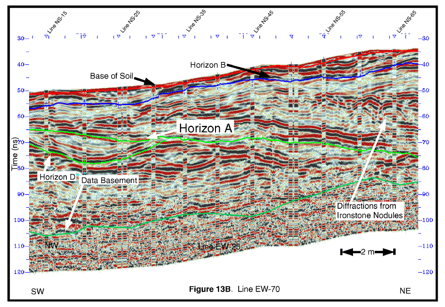
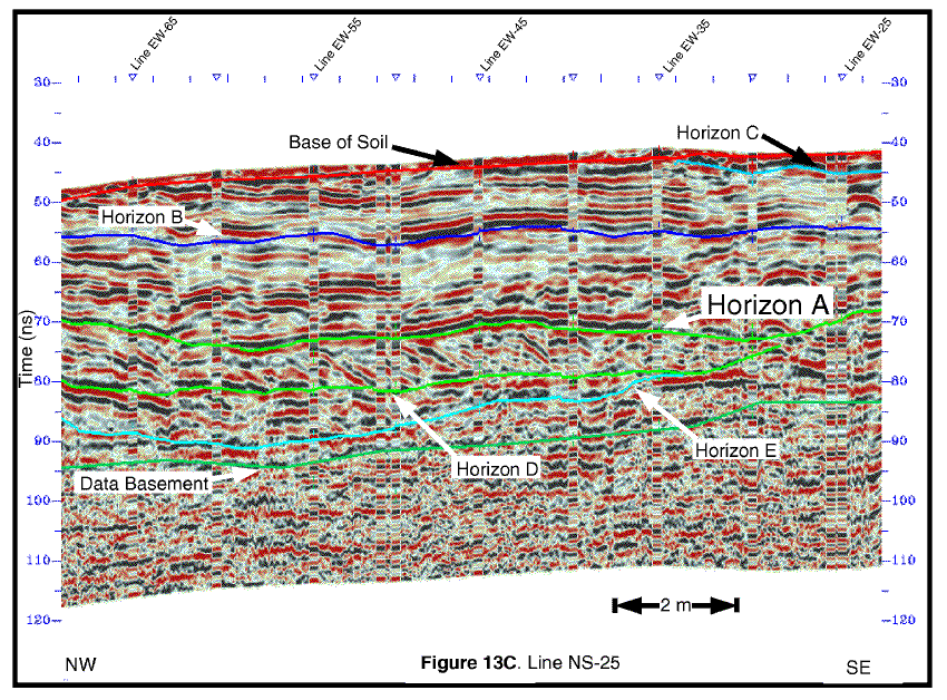
Figure 13C. A portion of the GPR profile from Line NS-25. Note how well the corssbedding is imaged below horizon A.
Some regions of Horizon A contain distinct diffractions, believed to be caused by ironstone nodules similar to what is seen in outcrop (Figure 13B).
The erosional base of convoluted trough and planar crossbedding, this horizon extends across the entire data grid (Figure 14B). In the southern portion of the gridded area, the top of the B-C interval (Figure 14A) is truncated by the modern erosional surface and an unknown amount of material has been removed by erosional processes.
The erosional base of sheet-like planar bedding, this horizon extends over only a portion of the data grid. Modern erosional processes have removed the upper surface of this interval. The C-soil interval (Figure 15A) is believed to have been deposited during the later stages of valley fill (Gibling et. al., 1993). Because of its planar nature, Horizon C was used as a datum (flattening horizon) in order to enhance lower reflection events.
Figure 15A. Isochron map of the interval from Horizon B to Horizon C. This is an interval of sheet-like planar bedding with an erosional base. The modern erosional surface truncates this interval and an unknown amount has been removed.
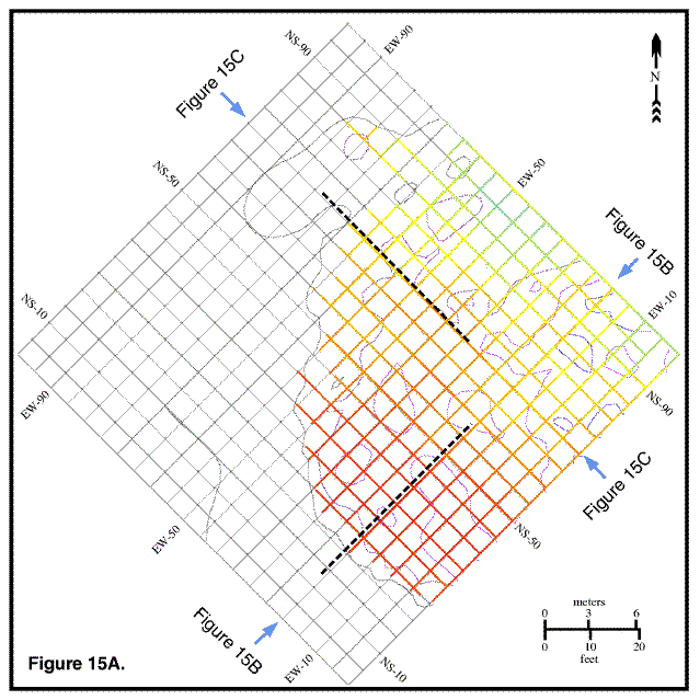
Figure 15B. A portion of the GPR profile from Line EW-20. The veolcity pull-down affecting the center of this profile is caused by a thicker soil cover along the surface.
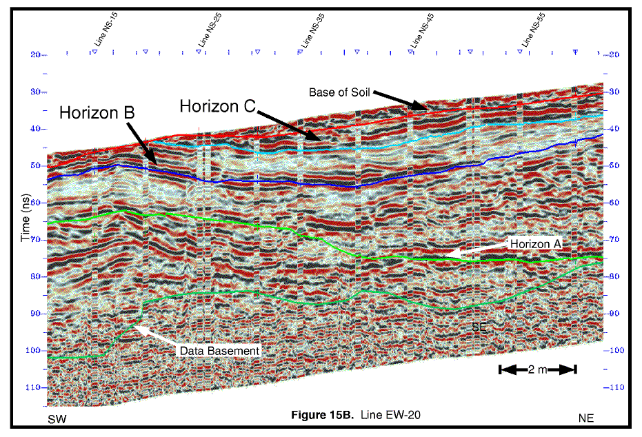
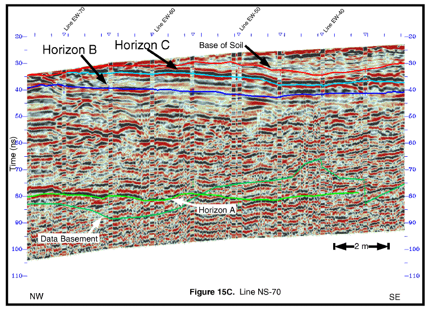
Figure 15C. A portion of the GPR profile from Line NS-70. Although the data basement crosses Horizon A along this line, the horizon was interpretable because of information from crossing lines. A larger version of this figure is available (156k).
This horizon is the erosional base of a small channel-fill. Its upper boundary is truncated by Horizon A. The D-A interval exhibits well-defined crossbedding (figures 16B and 16C). The general trend of the paleochannel is from NW to SE (Figure 16A).
Figure 16A. Isochron map of the interval from Horizon D to A. This interval is a small channel fill within the data grid. It is approximately 25 m x 6 m in extent and trends from NW to SE. It has an erosional base and a partially erosional top (truncated by Horizon A).
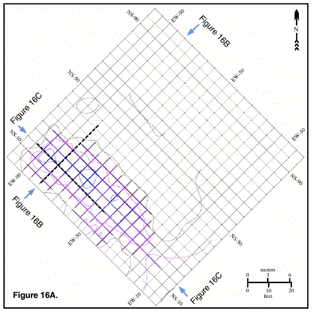
Figure 16B. A portion of the GPR profile from Line EW-80. Note the numerous other channel fills adjacent to and below Horizon D. Additional work will be necessary to further subdivide these intervals.

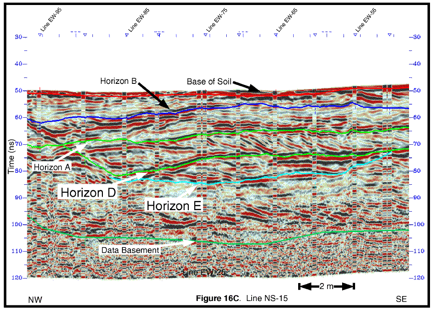
Figure 16C. A portion of the GPR profile from Line NS-15. Note the well defined crossbedding within the D to A interval.
This horizon is the erosional base of a small channel-fill. Its upper boundary is truncated by Horizons A and D. The interval above D exhibits well-defined crossbedding (Figures 17B and 17C). The general trend of the paleochannel is from NW to SE (Figure 17A).
Figure 17A. Isochron map of the interval from E to A and D. This interval is a small channel fill within the data grid. It is approximately 12 m x 4 m in extent and trends from NW to SE. It has an erosional base and a partially erosional top (truncated by Horizons A and D). Crossbedding is not as well defined within this interval as in the interval from Horizon D to A.
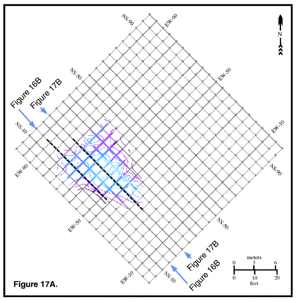
Figure 17B. A portion of the GPR profile from Line NS-25.
The following conclusions can be drawn from this study:
The authors wish to thank Neil Anderson, Mike Shoemaker, and Mike Roark of the University of Missouri, Rolla, for the use of UMR's equipment and their aid during data acquisition. Frank Gray provided land access. John Hopkins provided invaluable assistance in loading the horizon data into the contouring program. Field funding was provided by Tim Carr. The interpretation software for this project was provided by Landmark Graphics Corporation through an educational grant to the University of Kansas.
Collinson, J. D., 1986. Alluvial sediments; in, H. G. Reading, ed., Sedimentary Environments and Facies, Second Edition: Blackwell Scientific Publications, London, 615 p.
Davis, J. L., and A. P. Annan, 1989. Ground-penetrating radar for high-resolution mapping of soil and rock stratigraphy": Geophysical Prospecting, Vol. 37, p. 531-551.
Feldman, H. R., M. R. Gibling, A. W. Archer, W. G. Wightman, and W. P. Lanier, 1995. Stratigraphic architecture of the Tonganoxie paleovalley fill (Lower Virgilian) in northeast Kansas: American Assoc. of Petroleum Geologists, Bulletin, Vol. 79, No. 7, p. 1019-1043.
Gibling, M. R., H. R. Feldman, A. W. Archer, and W. P. Lanier, 1993. Sedimentology, stratigraphy and paleoflow patterns of the Tonganoxie Sandstone Member and related strata in northeast Kansas and southwest Missouri: Kansas Geological Survey, Open File Report 93-24, p. 3-1 to 3-39.
O'Conner, H. G., 1960. Geology and ground water resources of Douglas County, Kansas: Kansas Geological Survey, Bulletin 148, 200 p. [available online]
Winchell, R. L., 1957. Relationship of the Lansing Group and the Tonganoxie ("Stalnaker") Sandstone in south-central Kansas: Kansas Geological Survey Bulletin 127, p. 123-152. [available online]
Kansas Geological Survey, Energy Research
Placed online Sept. 1996
Comments to webadmin@kgs.ku.edu
The URL for this page is http://www.kgs.ku.edu/PRS/publication/OFR96_36/index.html