Kansas Geological Survey, Open-file Report 2004-67
by
Saibal Bhattacharya, Martin K. Dubois, and Alan P. Byrnes
Kansas Geological Survey, Lawrence, Kansas
KGS Open File Report 2004-67
This study follows the work summarized in KGS OFR 2004-66. In this previous study, the drainage area of Alexander D2 well (Figure 1A), located in Section 29, Township 27 South, Range 35 West, Grant County, Kansas, was modeled as if it produced only from the Council Grove (CG) reservoir. The type well profile (Figure 1B) shows that the Chase reservoir overlies the Council Grove reservoir. In most producing sections of the Hugoton and Panoma fields, two wells produce from the Chase Group (Hugoton Field) and a third produces from the Council Grove Group (Panoma Field). Though the Chase (Hugoton) directly overlies the Council Grove (Panoma), the two fields are regulated as separate fields. Three stages of development that followed in these fields can also be traced in our study area and consist of the the initial Hugoton well, the Alexander D-1 well Hugoton "parent" followed by the Alexander D-2, the Panoma well, and finally the Alexander D-3, a Hugoton infill well.
Figure 1a--Location of Alexander D-2 well compared to surrounding wells.
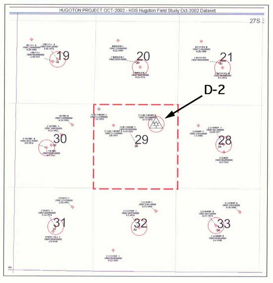
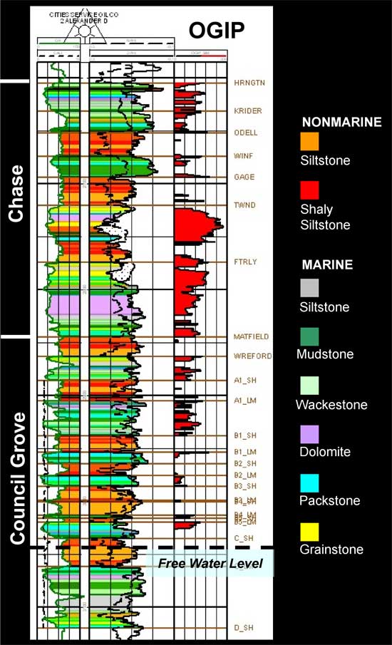
Figure 1b--Wireline log for Alexander D-2 annotated with lithofacies and original gas in place values.
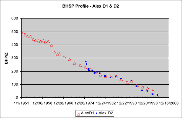
The estimated bottom-hole shut-in pressures (BHSPs), calculated from surface buildups, at Alexander D1 (referred here onward as D1) and Alexander D2 (referred here onward as D2) wells are compared in Figure 2. The plot shows that only during the initial year and half did D2 record BHSPs that were slightly higher than recorded at D1. Thereafter, the BHSPs at D1 and D2 almost march along in lock step till 1991, when Alexander D3 came online. This type of congruence between bottom hole shut-in pressures recorded in the Chase and Council Grove wells have been observed in other wells around D2 and over other parts of the Hugoton and Panoma fields leading to the speculation that these reservoirs are in hydraulic communication. This report summarizes the reservoir modeling of the Chase and Council Grove reservoirs as one system.
Figure 2--Estimated bottom-hole shut-in pressures (BHSPs).
The principal properties required for reservoir simulation studies are porosity, permeability, and initial water saturation (Sw). However, since Sw cannot be accurately estimated from wireline logs due to deep filtrate invasion during drilling, Sw must be estimated based on lithofacies dependent capillary pressure relationships (Dubois and others, 2003). Thus, projecting lithofacies in the 3D model space is a critical first step. For these exercises we have assumed that the layered flow units of both the Council Grove and Chase are laterally continuous across the entire unit and that the lithofacies within these units have the same degree of continuity. Properties in the model vary between layers but not within layers. This assumption is based upon the general observation that the lateral scale of major lithofacies bodies is much greater than the scale of the production unit being modeled.
The main flow units are relatively thin (2-10 meter) marine carbonates that are separated by thin (2-10 meter) nonmarine siltstones that have low permeability. The alternating layers were deposited as a series of stacked marine-nonmarine sedimentary cycles (Figure 1B). In the combined model (Chase and Council Grove), the 281 feet thick Chase group was also divided into one-foot layers, but since the Chase interval was not cored, lithofacies were predicted using a neural network model that was developed earlier (Dubois and others, 2003). Porosity at a one-foot scale was derived from wireline logs and was corrected based upon empirical relationships to core data. Permeability and water saturations were estimated at the one-foot scale given porosity and lithofacies using core-derived empirical relationships. Figure 1B shows the stratigraphic section for the Chase and Council Grove groups with wireline log curves. Color fill are lithofacies. Original gas in place (OGIP) is property-based volumetric for a free water level = 55 feet above sea level and bottomhole pressure = 465 psi.
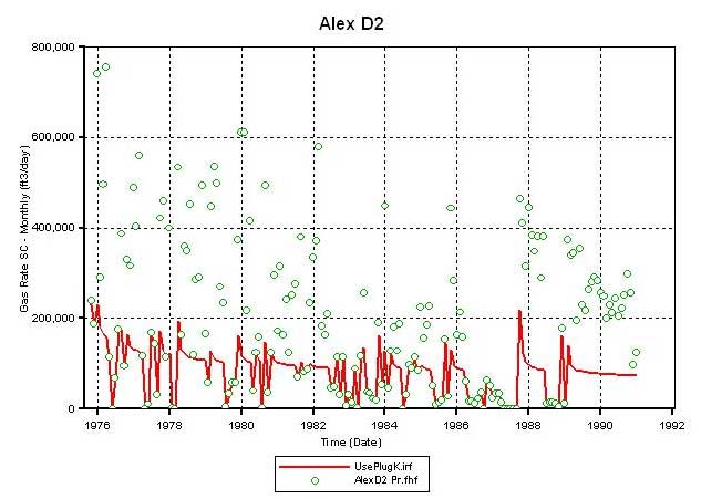
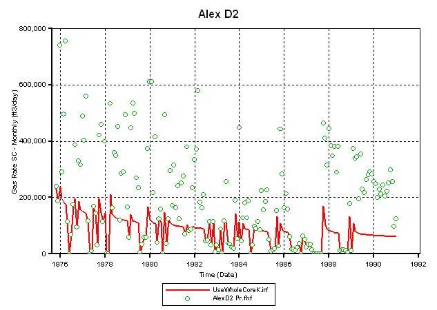
The initial simulation study (Figure 3A) modeled both the Chase and Council Grove reservoirs with the D1 well fractured and opened only in the Chase reservoir while the D2 well only fractured and opened in the CG reservoir. The period simulated extends from the completion of D1 (August 1951) to December 1990 (just before Alexander D3 came online). An upscaled model (as described in KGS-OFR No. 2004-66) was used in all the simulation runs discussed in this report. Based on shut-in pressure data, the initial starting pressure for the simulation was set to 465 psi. Figure 3A shows the calculated pressure distribution (using both north-south and east-west profiles) in November 1975. D2 came online in October 1975, and recorded an initial shut-in pressure of 259 psi. Thus, the model simulated shows differential pressure decline in the Chase layers and a production match at the D1 well (Figure 3B) but is unable to lower the reservoir pressure in the Council Grove reservoirs in the range of 250-260 psi. Though the model includes both the CG and the overlying Chase reservoirs, production at the D1 (Chase well) does not affect the pressure in the CG reservoir in the pre-D2 period. Also, the model is unable to match (Figure 3C) the production history at the D2 well from 1975 to 1990.
Figure 3a--Kxy derived from plug K-phi and Kv = .1 Kxy. Chase and Council Grove charge = 16.3 bcf; Chase charge = 13.7 bcf, Prod = 7.95 + 0.69 = 8.64 bcf, RF = 0.63; Council Grove charge = 2.5 bcf, Prod = 1.66 bcf, RF = 0.66.
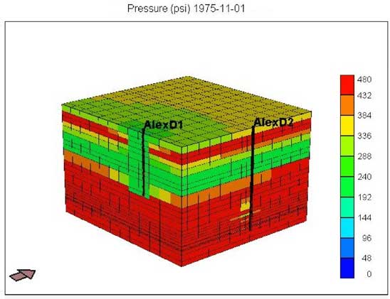
Figure 3b--Calculated production vs. actual production for Alexander D1.
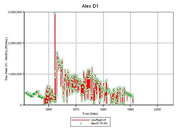
Figure 3c--Calculated production vs. actual production for Alexander D2.
One reason this model fails to match much of the D2 production may be that the matrix permeabilities used for the CG layers are too low. The layer permeabilities in this model were calculated by using facies-specific permeability-porosity correlations developed on data measured on core plugs. The core-plug based permeability estimation enables history matching of D1 while proves insufficient for D2. This prompted a closer examination of the permeability data by comparing plug based permeability with whole core permeability and also available DST permeability, and also the material balance evidences to confirm connectivity or lack of it between the Chase and CG reservoirs.
Permeability in both horizontal and vertical directions is very much scale dependent and the scale at which matrix permeability is measured, the one-inch diameter plug scale, is at the low end of the scale. Matrix (core plug) permeability is the starting point for the static 3D model since these data are readily available and also that facies-specific capillary pressure correlations used in water saturation estimates were developed from measurements taken on core plugs. Early in our simulation exercises we discovered that plug scale matrix permeability was insufficient for history matching reservoir performance and up to eight times matrix permeability was required. We have made some initial steps to provide geological explanations for the phenomena and a possible solution based on empirical data.
Permeability measurements available to us are at three scales, plug (Kp), whole core (Kwc) cylinders (approximately four inches in diameter and six inches in length), and drillstem test flow-based permeability (Kdst). Kp is generally less than Kwc in low permeability ranges and is equal to or lower than Kwc in high permeability ranges. Figure 4 shows examples of two Council Grove lithofacies having both Kp and Kwc for the same sample. The very fine-grained nonmarine sandstone has relatively low permeability and Kwc is 4.5 times greater than Kp while the more permeable grainstone Kwc is only 1.2 times Kp. Unfortunately we currently have insufficient data to make direct comparisons of Kwc and Kp on like samples. A method for developing an equation for estimating a multiplier for the transformation of Kp to Kwc is illustrated in Figures 5 to 7. In Figure 5, permeability is plotted against porosity for both Kp and Kwc and an exponentially fitted trend line was generated for each set. The two lines intersect at approximately 16% porosity and 1 millidarcy (md) permeability, while at 10% porosity Kwc is 0.5 md, 8.3 times Kpc of 0.06 md. At very low permeability, Kwc is more than two orders of magnitude greater than Kp.
Figure 4a--L-1 Nonmarine Siltstone and Sandstone; Whole Core Porosity (%) 10.8; Perm Max (md) 0.30; Plug Porosity (%) 11.9; Perm (md) 0.0667.
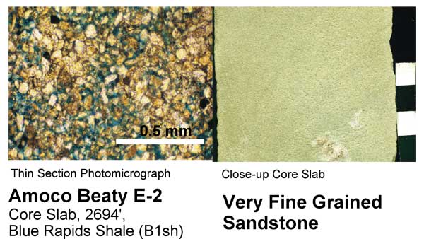
Figure 4b--L- 8 Grainstones. Whole Core Porosity (%) 18.8; Perm Max (md) 39.0; Plug Porosity (%) 21.2; Perm (md) 32.3.
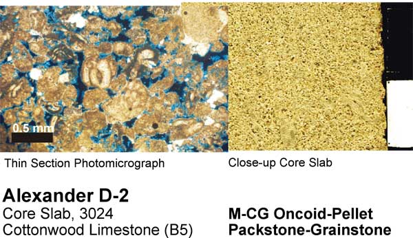
Figure 5--Plug and whole core comparison.
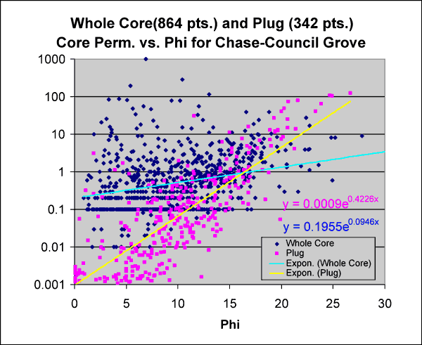
Figure 6--Multiplication factor required to estimate whole core k from plug k.
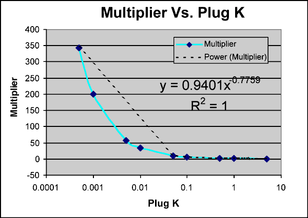
Figure 7--Multiplier calculation.
|
|||||||||||||||||||||||||||||||||||||||||
|
Recommendation Plug k < 0.00245, K = 100 * Plug k 0.00245 < Plug k < 0.922, K = y * Plug k (use y = 0.9401x-0.7759 where y = multiplier and x = plug k) Plug perm > 0.922, Plug = Whole Core |
||||||||||||||||||||||||||||||||||||||||
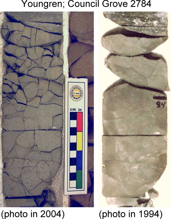
It would appear from work to date that whole core permeability could be more appropriate than plug permeability, but this would imply that the microfracturing that is required for higher permeability in whole core is also present in the reservoir in all lithofacies and is pervasive and not merely induced in the whole core by the coring operation. Though not obvious or pervasive in core we do see some micro and larger scale fractures. Figure 8 shows microfractures in a nonmarine siltstone paleosols. The 1994 photo is of the core very soon after being cored using an underbalanced foam system to minimize filtrate invasion. Small microfractures that may be outlines of peds are barely visible in the 1994 photo but are readily apparent in the 2004 photo. Time (weathering) and handling have aided the disintegration. These microfractures may be natural and may have contributed to permeability at scales larger than plugs. Larger scale vertical fractures partially filled with cement are common, though not abundant in nearly every carbonate layer in every core, but much less abundant in the nonmarine siltstones. These fractures likely provide additional permeability at scales larger than whole core.
Figure 8--Simulation model requires kmod = 8 x kmatrix-plug to match production. Is there geologic-based rationale for this? Core plug matrix k is minimum permeability. Whole core k is up to 1 order of magnitude higher than plug due to microfractures, either natural or induced.
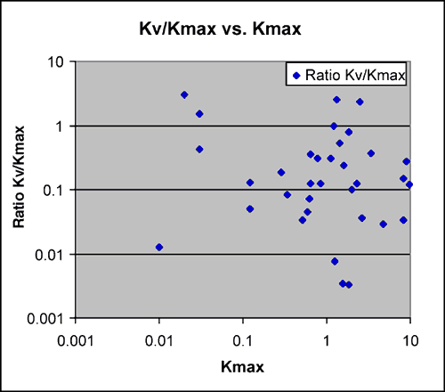
A plot (Figure 9) of Kdst versus whole core and plug permeability for the same interval shows consistently lower permeability than would be suggested by whole core. Further investigation is needed on this subject. In early models vertical permeability (Kv or Kz) was estimated at 0.1 times horizontal permeability (Kxy). A plot of the ratio of Kv to maximum horizontal permeability (Kmax) versus Kmax for whole core is shown in Figure 10. The core data available suggests that a Kv/Kmax ratio of 0.25 may be more appropriate.
Figure 9--Arithmetic average core k (39 whole core and 6 plug k) cross plotted with average DST k (45 DST's).
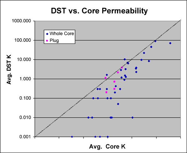
Figure 10--Kz/Kxy used so far is 0.1. Preliminary work on limited core data suggests that 0.25 may be more appropriate.
| Median | Mean | Count | |
|---|---|---|---|
| Kz/Kxy (all) |
0.273 | 8.141 | 89 |
| Kz/Kxy (no value > 1) |
0.231 | 0.318 | 77 |
| Kz/Kxy (no value > 1 or < 1) |
0.254 | 0.354 | 66 |
Shut-in pressures and cumulative gas production (Gp) from D1 and D2 were used for material balance studies to determine if the above wells were draining from a "single bottle," i.e., a system where the Chase and CG reservoirs were in communication. Figure 11 displays the plot of bottom-hole shut in (BHP/z) pressure and cumulative gas production from D1 from 1951 to Dec 1974 (just before D2 came online). The data plots on a good linear trend and the calculated original-gas-in-place (OGIP) is 9.5 bcf for the drainage volume in communication with D1. If D2 also produced from the same "bottle" as D1, then a plot of pressure (average reservoir pressure of drainage connected to D1 and D2) and the total cumulative production (from D1 and D2) from 1975 to Jan 1991 (before D3 came online) would follow the same linear trend of pre-1975 data thereby resulting a calculated OGIP that is close to 9.5 bcf.
Figure 11--Bottom-hole shut-in pressure vs. cumulative gas production.
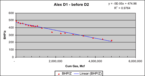
Material balance formulation:
P/z = Pi/zi - (Pi/zi) * (Gp/G)
Total gas reserves:
Pi/zi = 474 psi
G = 9,499,200 mcf
Gp = 4,803,477 mcf
Rf = 0.51
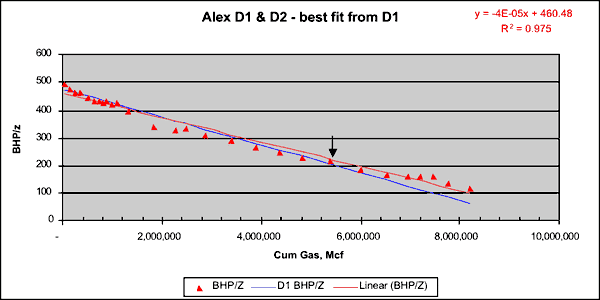
Though there are two producing wells after 1975, Figure 2 shows that it is not unreasonable to use D1 reservoir pressure history as the representative average pressure profile (for both D1 and D2) between 1975 and 1991. Figure 12 shows the plot of average reservoir pressure (BHP/z) and total cumulative production (from D1 and D2) plotted till Dec 1990. We get another linear trend and the OGIP is calculated at 11.5 bcf, which being higher than that obtained from pre-1975 data (Figure 11) indicates that the post-1975 data do not plot on the same linear trend defining the pre-1975 data. The data plotted in Figure 13 is identical to Figure 12. The only addition is the blue line that shows the trend of the pre-1975 data. This plot clearly shows that once D2 came on line, additional production resulted in less than expected decline in reservoir pressure as predicted by data from D1 only (pre-1975). That the red triangles stray upward and away from the blue line indicates that additional energy was added to the reservoir post-1975. This happens when fluid is injected into a reservoir. However, since no fluid was injected in the CG or Chase after 1975, one explanation for the red triangles straying up and away from the blue line is that D2 opened up some new drainage that was not connected with D1. If D2 did in fact open up additional drainage, then pre-1975 data can not be plotted along with post-75 data as a part of the same MB calculations because that would violate one the basic MB assumptions--i.e., the drainage volume must remain constant.
Figure 12--Average reservoir pressure (BHP/z) and total cumulative production. If D1 and D2 share the same drainage, then the above estimated OGIP of 11.5bcf must be confirmed by pre-1975 data (i.e. before D2 came online).
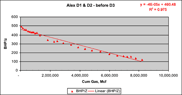
Material balance formulation:
P/z = Pi/zi - (Pi/zi) * (Gp/G)
Total gas reserves:
Pi/zi = 460.48 psi
G = 11,512,000 mcf
Gp = 8,191,438 mcf (till Dec. 1990--D1 and D2)
Rf = 0.71 (as of Dec. 1990)
Additional recoveries since Dec. 1990:
D1 prod. from Dec. 1990 to Mar. 2004 = 852,141 mcf
D2 prod. from Dec. 1990 to Mar. 2004 = 1,420,650 mcf
Prod. from D3 = 702,347 mcf
Total additional prod. since Dec. 1990 (D1 and D2) = 2,272,791 mcf
Total additional prod. since Dec. 1990 (D1, D2 and D3) = 2,975,138 mcf
Final lease RF--March 2004 = 0.97
(if all three drained same drainage area)
Figure 13--Average reservoir pressure (BHP/z) and total cumulative production.
Thus, MB calculations for the D2 drainage area are beset with a problem. The additional (recent) well seems to connect to new drainage volume unseen by the previous well. This does not mean that D2's drainage is exclusive of D1's. Their drainages perhaps overlap, but D2 connects to additional drainage not earlier connected to D1. It was initially hoped that lacking reliable log-derived Sw, MB calculations would provide guidance/estimation of OGIP. However, this exercise shows the limitations of MB calculations and the care that must be invested before application of OGIP estimates based on MB calculations.
Previously mentioned simulation results indicate that plug-data-based permeability-porosity correlations were sufficient to match production history in Chase but not in CG reservoir wells. Figure 14A shows the upscaled layer Sw and permeabilities in Chase and CG estimated by using plug-based permeability data. It becomes apparent that the Chase layers have more gas than the CG, but Chase production is driven by higher layer permeabilities than the CG. Thus following observations between whole core permeability and plug permeability data (Figure 7), the horizontal permeability (Kxy) over a half-foot interval was multiplied by 100 if its plug-derived value was less than 0.00245 md, while a multiplier was calculated, using the formula y=0.9401*x(-0.7759) [where y is the multiplier and x is the plug-derived permeability], when the plug-based permeability varied between 0.00245 md and 0.922 md. For plug-based permeability values greater than 0.922 md, a multiplier of 1 was used. Also, based on available whole core data, the vertical permeability for each half-foot layer was assumed to be 0.25 the Kxy. The resultant layer permeabilities are summarized in Figure 14B.
Figure 14A--Plug-based permeability estimates, no permeability multiplier applied. Chase layers indicated by green, Council Grove layers by yellow.
| Kv/Kxy multiplier = 0.1 | ||||||
| Upscl H ft | Upscl Phi | UpScl Sw | UpScl K hor md | UpScl Kv md | ||
|---|---|---|---|---|---|---|
| 1 | HRNGTN | 26.5 | 0.089 | 0.33 | 1.182 | 3.34794E-07 |
| 2 | KRIDER | 19.5 | 0.069 | 0.46 | 0.042 | 1.34307E-07 |
| 3 | ODELL | 21.5 | 0.071 | 0.99 | 0.002 | 0.000125028 |
| 4 | WINF | 19.5 | 0.058 | 0.41 | 0.356 | 1.19645E-13 |
| 5 | GAGE | 26.5 | 0.076 | 0.99 | 0.054 | 0.000159669 |
| 6 | TWND | 33.5 | 0.169 | 0.38 | 55.238 | 0.004026007 |
| 7 | HOLMESVILLE | 18.5 | 0.099 | 0.99 | 0.250 | 0.000192849 |
| 8 | FTRLY | 22.5 | 0.144 | 0.28 | 11.822 | 0.013852189 |
| 9 | L_FTRLY | 47.5 | 0.109 | 0.43 | 0.289 | 1.04493E-05 |
| 10 | MATFIELD | 17.5 | 0.076 | 0.99 | 0.004 | 0.000172546 |
| 11 | WREFORD | 22.5 | 0.096 | 0.51 | 0.259 | 5.09112E-05 |
| 12 | A1_SH | 19 | 0.079 | 0.91 | 0.220 | 0.000146295 |
| 13 | A1_LM | 32 | 0.103 | 0.54 | 0.457 | 4.77417E-05 |
| 14 | B1_SH | 15.5 | 0.080 | 0.99 | 0.007 | 0.000274647 |
| 15 | B1_LM | 10 | 0.071 | 0.78 | 0.824 | 1.90486E-06 |
| 16 | B2_SH | 11 | 0.073 | 0.99 | 0.017 | 0.000112545 |
| 17 | B2_LM | 9.5 | 0.091 | 0.79 | 0.160 | 0.003293057 |
| 18 | B3_SH | 13 | 0.084 | 0.99 | 0.016 | 0.000239957 |
| 19 | B3_LM | 1 | 0.086 | 0.72 | 0.189 | 0.012473465 |
| 20 | B4_SH | 11.5 | 0.080 | 0.99 | 0.027 | 0.000192878 |
| 21 | B4_LM | 2.5 | 0.134 | 0.63 | 5.211 | 0.12593811 |
| 22 | B5_SH | 3.5 | 0.070 | 0.99 | 0.001 | 0.000122015 |
| 23 | B5_LM | 14.5 | 0.138 | 0.77 | 7.063 | 0.005252614 |
| 24 | C_SH | 26 | 0.070 | 0.99 | 0.002 | 0.000148729 |
| 25 | C_LM | 57.5 | 0.094 | 1.00 | 2.795 | 7.23571E-05 |
Figure 14B--Plug-based permeability estimates, selective permeability multiplier applied. Chase layers indicated by green, Council Grove layers by yellow.
| Kv/Kxy multiplier = 0.25 | ||||||
| Upscl H ft | Upscl Phi | UpScl Sw | UpScl K hor md | UpScl Kv md | ||
|---|---|---|---|---|---|---|
| 1 | HRNGTN | 27 | 0.089 | 0.33 | 1.401 | 8.52512E-05 |
| 2 | KRIDER | 20 | 0.069 | 0.46 | 0.261 | 3.44329E-05 |
| 3 | ODELL | 22 | 0.071 | 0.97 | 0.151 | 0.031445022 |
| 4 | WINF | 20 | 0.058 | 0.41 | 0.481 | 3.06782E-11 |
| 5 | GAGE | 27 | 0.076 | 0.90 | 0.213 | 0.039828652 |
| 6 | TWND | 34 | 0.169 | 0.19 | 55.345 | 0.280904773 |
| 7 | HOLMESVILLE | 19 | 0.099 | 0.64 | 0.422 | 0.045080797 |
| 8 | FTRLY | 23 | 0.144 | 0.28 | 11.900 | 0.416917007 |
| 9 | L_FTRLY | 48 | 0.109 | 0.43 | 0.583 | 0.002607391 |
| 10 | MATFIELD | 18 | 0.076 | 0.98 | 0.202 | 0.040509001 |
| 11 | WREFORD | 23 | 0.096 | 0.51 | 0.523 | 0.012327338 |
| 12 | A1_SH | 19.5 | 0.079 | 0.90 | 0.392 | 0.035447834 |
| 13 | A1_LM | 32.5 | 0.103 | 0.54 | 0.760 | 0.011493021 |
| 14 | B1_SH | 16 | 0.080 | 0.99 | 0.254 | 0.055176391 |
| 15 | B1_LM | 10.5 | 0.071 | 0.78 | 1.078 | 0.000498971 |
| 16 | B2_SH | 11.5 | 0.073 | 0.98 | 0.169 | 0.028966931 |
| 17 | B2_LM | 10 | 0.091 | 0.79 | 0.558 | 0.128446483 |
| 18 | B3_SH | 13.5 | 0.084 | 0.99 | 0.270 | 0.050936456 |
| 19 | B3_LM | 1.5 | 0.086 | 0.72 | 0.646 | 0.161548365 |
| 20 | B4_SH | 12 | 0.080 | 0.99 | 0.250 | 0.04467553 |
| 21 | B4_LM | 3 | 0.134 | 0.63 | 5.286 | 0.491584825 |
| 22 | B5_SH | 4 | 0.070 | 0.99 | 0.139 | 0.034861456 |
| 23 | B5_LM | 15 | 0.138 | 0.77 | 7.217 | 0.256295099 |
| 24 | C_SH | 26.5 | 0.070 | 0.99 | 0.153 | 0.037897379 |
| 25 | C_LM | 58 | 0.094 | 1.00 | 3.041 | 0.016952937 |
Figure 15A shows the differential pressure depletion in the Chase and CG reservoirs as of November 1975. It indicates that in the current model, with layer permeabilities based on whole core observations, Chase production (from D1) leads to depletion of reservoir pressure in CG. In October 1975, the CG pressure, estimated from D2, is around 260 psi (Figure 15B). However, the current model predicts that the CG pressure is mostly between 250 psi (in D2's vicinity) to 370 psi, indicating that further fine tuning is required. Figure 3B shows that the current model matches production from D1. However, it falls significantly short in matching D1 production (Figure 3C).
Figure 15a--Selective multiplier applied to estimate Kxy (plug to whole core) and Kv = .25 Kxy. Modeled pressure depletion as of November 1975.
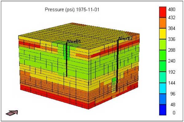
Figure 15b--Reservoir pressure from shut-in tests.
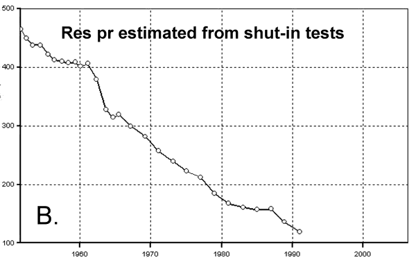
Figure 15c--Calculated production vs. actual production for Alexander D2.
Figure 3a--Kxy derived from plug K-phi and Kv = .1 Kxy. Chase and Council Grove charge = 16.3 bcf; Chase charge = 13.7 bcf, Prod = 7.95 + 0.69 = 8.64 bcf, RF = 0.63; Council Grove charge = 2.5 bcf, Prod = 1.66 bcf, RF = 0.66.
Figure 16a--Calculated production vs. actual production for Alexander D1.
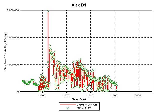
Figure 16b--Calculated production vs. actual production for Alexander D2.
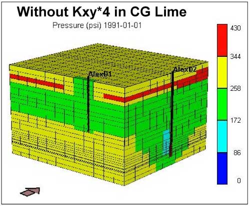
To improve the production match at D2, the permeability (Kxy) multiplier of 4 was employed selectively on the limestone layers in CG. Figure 17 compares the results of this permeability increase with that from the case when it was not applied. The increase in lime permeability in CG results in an increase in the simulator calculated gas production at D2 (Figures 17A and 17C) and therefore lower average reservoir pressure in CG by January 1991 (Figures 17B and 17D). Though the simulator-calculated gas production increased, it still is far from matching the historic production. Thus, it appears that at the given OGIP charge in the CG (as of October 1975) the current permeability distribution, despite using whole core values and a multiplier of 4 in the limestone layers, is insufficient to produce the gas volumes recorded at D2.
Figure 17a--Calculated production vs. actual production for Alexander D2 where permeability multipled by 4 in Council Grove limestones.
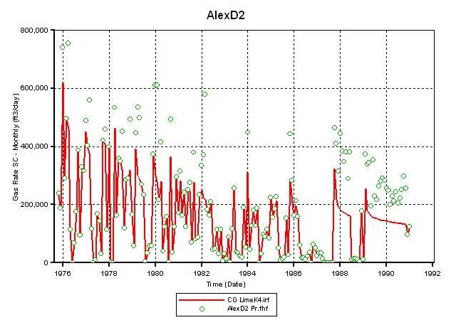
Figure 17b--Block diagram showing average reservoir pressure; permeability multipled by 4 in Council Grove limestones.
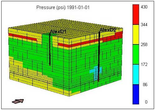
Figure 17c--Calculated production vs. actual production for Alexander D2 without permeability adjustment.
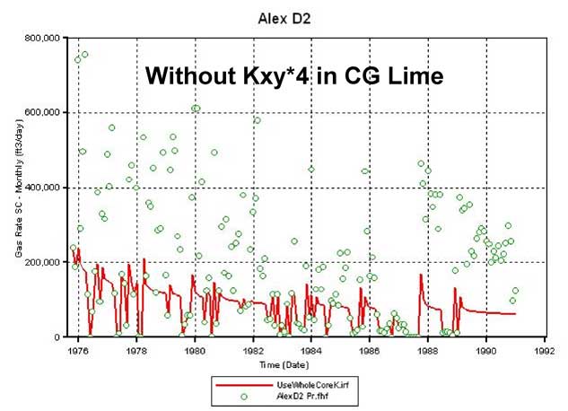
Figure 17d--Block diagram showing average reservoir pressure; permeability not adjusted.
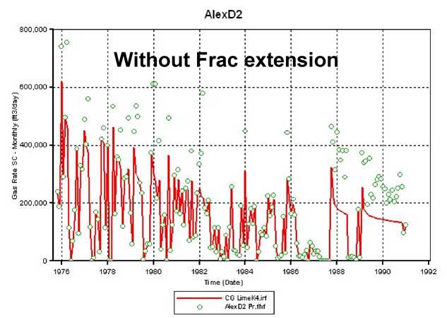
Not knowing the exact nature of connectivity between the Chase and the CG reservoirs, the hydraulic fracture in D2 was extended first into the bottom 2 and then into the bottom 4 Chase layers. Figure 18A plots the simulator-calculated cumulative gas production from D2 when the fracture is extended to 2 layers (broken red line) and 4 layers (green line) in the Chase. Extending the D2 fracture into Chase increases production but is still insufficient to match the historic volumes at D2 (Figure 18B). However, such a fracture extension does not interfere with D1 production (Figure 18C). Results from this run also show that extending the D2 fracture into the Chase (bottom layers) enables D2 to produce some of the Chase gas and come closer to matching the historic production but in the process leads to higher average reservoir pressures in CG. Thus, extending the D2 fracture into the Chase is not helpful in improving the simulator performance (production and average reservoir pressure match) for D2.
Figure 18a--Cumulative production for Alex D2.
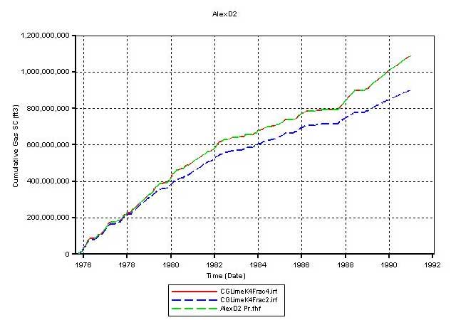
Figure 18b--Calculated production vs. actual production for Alexander D1; adjustment to D2 does not harm D1 match.
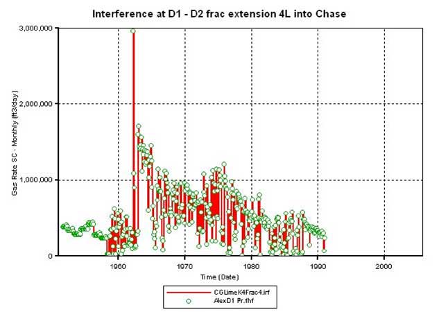
Figure 18c--Calculated production vs. actual production for Alexander D2 with fracture adjustment.
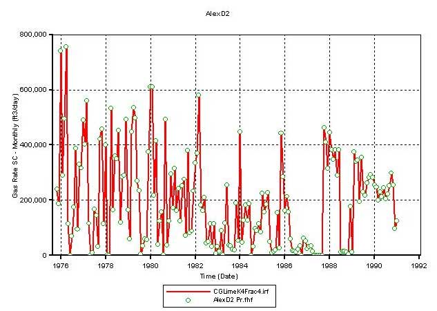
Figure 18d--Calculated production vs. actual production for Alexander D2 without adjustment.
It appears from these experiments additional studies are necessary to develop a better understanding about the connectivity between the Chase and Council Grove reservoirs, the volumes of OGIP in Chase and CG before start of production, and the permeability distribution, especially in the CG reservoir layers.
Kansas Geological Survey, Energy Research
Placed online May 16, 2005
Comments to webadmin@kgs.ku.edu
The URL for this page is HTTP://www.kgs.ku.edu/PRS/publication/2004/OFR04_67/index.html