Kansas Geological Survey, Open-file Report 2004-64
by
Martin K. Dubois1, Geoffrey C. Bohling1, and Swapan Chakrabarti2,
1Kansas Geological Survey, Lawrence, Kansas
2Department of Electrical Engineering and Computer Science, University of Kansas, Lawrence, Kansas
KGS Open File Report 2004-64
Feb. 2005
Facies classification, assigning a rock type or class to specific rock samples, on the basis of measured rock properties is a fundamental step in geologic interpretations and a variety of useful classification schemes may be employed. In this experiment three statistically based classifiers, Bayesian, fuzzy logic, and feed forward, back propagating artificial neural networks (ANN), were tested in a rock facies classification problem. The data set consisted of approximately 3600 samples with known rock facies class with each sample having seven measured or derived properties. This rock facies classification problem is part of a geologic modeling project of the Council Grove Group that is being undertaken at the Kansas Geological Survey (KGS). The Council Grove is a rock stratigraphic interval that produces gas in the Panoma Gas Field in southwest Kansas. The sample set was divided into two sets, one for training the classifiers and one for testing the ability of the classifier to correctly assign classes. The ANN significantly outperformed the other two classifiers.
Classification of lithofacies and their accurate representation in a 3D cellular geologic model is required for reservoir analysis of the Council Grove Group because permeability and fluid saturations for a given porosity and height above free water vary considerably among lithofacies (Byrnes, Dubois and Magnuson, 2001; Dubois, et al., 2003a). The conventional method of manually assigning lithofacies in half-foot segments of a 200-foot interval on a well-by-well basis is impractical due to the immense volume of data being considered (500 wells). Developing an efficient method to accurately assign lithofacies to half-foot intervals in hundreds of wells is critical to the KGS study. Preliminary work indicates that properly trained ANNs are effective tools for assigning lithofacies to rock intervals based on measured and derived properties (Dubois, et al., 2003a,b). The objective of this project is to investigate more rigorously the use of ANNs as well as explore alternate classification methods.
Classification of rocks is fundamental to geology and a variety of useful classification schemes may be employed, depending upon the circumstances. Rocks of the Council Grove Group fall into the large category of sedimentary rocks that, in this project, is subdivided into eight rock types or facies. The spectrum of rocks in this study is a continuum that could be lumped or split in many ways. We settled on eight classes (facies) in the KGS study by balancing three objectives: (1) maximum number of facies recognizable by petrophysical wireline logs; (2) minimum number needed to accurately represent the physical variability of the reservoir; and (3) class distinction of petrophysical properties at the pore and core plug level.
Facies and rocks in general have a large number of physical and chemical properties that can be used for classification. In oil and gas wells the most readily available properties related to the rocks encountered are measurements made by petrophysical tools lowered into the eight-inch wellbore after a well is drilled. Digital information is recorded at half-foot increments from a variety of devices that measure a number of physical properties (porosity, natural gamma radiation, resistivity, photoelectric effect). These properties, their combinations or derivatives, are possible elements of feature vectors spaced at a half-foot increment in a wellbore. Five feature elements measured by wireline logs considered for this project are natural gamma ray radiation (GR), neutron and density porosity average (PHI), neutron porosity and density porosity difference (N-D), photoelectric effect (PE), and apparent true resistivity (Rta), illustrated in Figure 1.
Figure 1--Wireline log with input variables (feature elements) for a 250-foot oportion of the Council lGrove Group. Color indicates known lithofacies (class).
Different facies have characteristic wireline log "signatures", a combination of the responses measured by the petrophysical tools, which allow one to differentiate facies. Two other feature elements derived from other geologic data are geologic constraining variables (GCV), nonmarine-marine (NM-M) and relative position (RPos). NM-M is determined from formation tops and bases and RPos is the position of a particular sample with respect to the base of its respective nonmarine or marine interval. These two important variables help to incorporate geologic knowledge into the variable mix.
The PE is available for only five of the eight wells in the training set shown in Figure 2. This PE availability ratio approximates that of the PE availability of the entire 515 well set. Since PE is a powerful facies discriminating variable it will be used where available in later applications of the classifiers. Thus two models for each type of classifier, one using the PE (PE) and one not using PE (NoPE), were developed and tested.
Figure 2--Map showing location of eight wells in training set (large triangles) and 515 wells without lithofacies information (without triangles). Dimensions of map are approximately 96 by 84 miles (150 by 135 km).
This project involves fuzziness at many levels, yet the final desired output, facies class, is crisp (discrete). Facies class boundaries are inherently fuzzy because the rocks in this system are comprised of varying amounts of basically four mineral components, calcite, dolomite, quartz, and clay, in a continuum. In a sense, crisp class boundaries are somewhat arbitrary and subjective. Furthermore, properties measured by wireline logs are fuzzy on three levels. First, for each class there is a fairly wide range of responses for each measured property and the feature spaces of each property have significant overlap between classes (Figure 3 and Table 1). Second, wireline log measurements at the half foot interval are actually an average of the properties over as much as several feet, a physical limitation inherent in the wireline tools. Third, varying borehole conditions influence measurements by the wireline tools and the effects of these perturbations cannot be effectively corrected or normalized.
Figure 3--Histograms of GR, one of the input variables, by lithofacies (class).
Table 1--Test and training set lithofacies (class) and feature vector variable statistics.
| Lithofacies and Variable Statistics | GR | Nphi-Dphi | PE | Avg Phi | Rta | Rel Pos to Base | ||||||||
|---|---|---|---|---|---|---|---|---|---|---|---|---|---|---|
| Lith Code | Lithofacies | Count | Mean | StdDev | Mean | StdDev | Mean | StdDev | Mean | StdDev | Mean | StdDev | Mean | StdDev |
| All | All | 3647 | 63.68 | 29.48 | 4.89 | 4.93 | 3.75 | 0.76 | 11.84 | 5.06 | 5.69 | 4.30 | 0.53 | 0.28 |
| 1 | NM Silt & Sand | 950 | 70.47 | 12.63 | 5.58 | 4.66 | 3.21 | 0.38 | 12.84 | 3.78 | 3.72 | 1.35 | 0.48 | 0.24 |
| 2 | Nm ShlySilt | 817 | 78.62 | 14.45 | 6.81 | 5.78 | 3.30 | 0.49 | 16.18 | 5.19 | 3.85 | 1.28 | 0.56 | 0.32 |
| 3 | Mar Shale & Silt | 280 | 87.20 | 45.21 | 6.05 | 3.62 | 3.73 | 0.49 | 11.77 | 3.03 | 6.27 | 2.09 | 0.40 | 0.19 |
| 4 | Mdst/Mdst-Wkst | 251 | 59.43 | 36.16 | 5.17 | 3.92 | 4.09 | 0.54 | 8.58 | 3.38 | 7.86 | 2.98 | 0.58 | 0.28 |
| 5 | Wkst/Wkst-Pkst | 600 | 53.04 | 30.67 | 2.96 | 3.51 | 4.25 | 0.64 | 7.90 | 3.31 | 8.30 | 4.60 | 0.51 | 0.28 |
| 6 | Sucrosic (Dol) | 147 | 42.24 | 18.41 | 6.30 | 3.93 | 3.77 | 0.56 | 13.01 | 4.69 | 3.30 | 1.59 | 0.67 | 0.24 |
| 7 | Pkst/Pkst-Grnst | 459 | 40.16 | 30.69 | 2.37 | 3.78 | 4.61 | 0.66 | 9.03 | 4.08 | 8.76 | 7.80 | 0.58 | 0.30 |
| 8 | Grnst/PA Baff | 143 | 36.89 | 15.81 | 1.22 | 6.41 | 4.44 | 1.00 | 10.50 | 4.36 | 6.09 | 4.60 | 0.56 | 0.32 |
This study assumed that all data collected and organized in conjunction with the larger Panoma modeling project is accurate and appropriately screened. Classification models for the two situations, with PE and without PE, were trained and tested in the same manner. The experiment involved the following broad steps: (1) data preparation; (2) design, train and test classifiers using discriminant analysis with Bayes' rule; (3) design, train and test fuzzy logic classifiers; (4) design, train and test a conventional feed forward, back propagating artificial neural networks (ANN); and (5) analyze and compare results from the three classifiers using metrics designed to meet the objectives of the classification problem.
The driving force in the search for an efficient classification tool is the need to automate the process. Since rock properties controlling gas production overlap, facies boundaries are blurred, and measuring devices tend to average, a high degree of absolute correct classification is not anticipated. Having a facies classification that is close to the actual may be judged as satisfactory because the facies are nearly a continuum (reflected in the numeric class code). In addition to being correct or nearly correct it is important that the number of a particular facies predicted by any classifier be relatively close to that in the overall population in order that the ultimate model accurately represents facies distribution. The accurate representation of the main gas pay zones, facies 6, 7 and 8, is also important and needs to be measured. To accomplish these objectives, six metrics were used:
| 1. Percent correct for all facies | (Correct) |
| 2. Percent correct for facies 6-8 | (F678Correct) |
| 3. Percent within one facies* | (Close ±1F) |
| 4. Percent within one facies* for facies 6-8 | (F678Close ±1F) |
| 5. Ratio of predicted facies to actual facies count by facies | (%Actual-all) |
| 6. Standard deviation of metric 5 across the spectrum of facies | (SD%All) |
| *Due to certain circumstances, special rules are applied: F2 is not one facies from F3 and vice versa; F8 is considered one facies from both F7 and F6; F7 is considered one facies from F5, F6 and F8). | |
The training and testing set consists of 3647 examples having known, core-defined facies classes that are associated with feature vectors having either six or seven elements. The examples are from eight wells across the field selected on the basis of stratigraphic and geographic coverage, availability of appropriate wireline logs, and availability of core analysis data. The examples were randomly split into two sets, 2/3rd for training and 1/3rd for testing (Table 2). The same set splits were used for training and testing all classifiers. Other statistics for the data are in Table 1 and Table 5. Examples of feature vectors by facies (class) are shown in Table 3.
Table 2--Randomly split data sets and their facies counts.
| Complete sample set | ||||
| Facies | All | PE | NoPE | Ratio PE |
|---|---|---|---|---|
| 1 | 950 | 549 | 401 | 0.58 |
| 2 | 817 | 539 | 278 | 0.66 |
| 3 | 280 | 170 | 110 | 0.61 |
| 4 | 251 | 152 | 99 | 0.61 |
| 5 | 600 | 422 | 178 | 0.70 |
| 6 | 147 | 87 | 60 | 0.59 |
| 7 | 459 | 261 | 198 | 0.57 |
| 8 | 143 | 94 | 49 | 0.66 |
| 3647 | 2274 | 1373 | 0.62 | |
| 2/3 train | ||||
| Facies | All | PE | NoPE | Ratio PE |
| 1 | 639 | 377 | 262 | 0.59 |
| 2 | 532 | 380 | 152 | 0.71 |
| 3 | 180 | 109 | 71 | 0.61 |
| 4 | 172 | 103 | 69 | 0.60 |
| 5 | 399 | 279 | 120 | 0.70 |
| 6 | 94 | 55 | 39 | 0.59 |
| 7 | 323 | 190 | 133 | 0.59 |
| 8 | 92 | 61 | 31 | 0.66 |
| 2431 | 1554 | 877 | 0.64 | |
| 1/3 test | ||||
| Facies | All | PE | NoPE | Ratio PE |
| 1 | 311 | 172 | 139 | 0.55 |
| 2 | 285 | 159 | 126 | 0.56 |
| 3 | 100 | 61 | 39 | 0.61 |
| 4 | 79 | 49 | 30 | 0.62 |
| 5 | 201 | 143 | 58 | 0.71 |
| 6 | 53 | 32 | 21 | 0.60 |
| 7 | 136 | 71 | 65 | 0.52 |
| 8 | 51 | 33 | 18 | 0.65 |
| 1216 | 720 | 496 | 0.59 | |
Table 3--Sample data set showing facies and seven element feature vectors
| Facies | Log10GR | Avg Phi | Log10RTA | PE | N-D | M-NM | RPb |
|---|---|---|---|---|---|---|---|
| 1 | 1.796 | 15.35 | 0.296 | 3.1 | 4.7 | 1 | 0.340 |
| 5 | 1.808 | 9.30 | 0.754 | 4.0 | 7.2 | 2 | 0.776 |
| 7 | 1.754 | 3.25 | 0.951 | 5.0 | 2.1 | 2 | 0.552 |
| 3 | 1.828 | 14.30 | 0.661 | 3.4 | 9.2 | 2 | 0.328 |
| 2 | 1.866 | 21.90 | 0.537 | 3.6 | -1 | 1 | 0.051 |
| 5 | 1.685 | 6.25 | 0.979 | 3.4 | 0.5 | 2 | 0.739 |
| 7 | 1.386 | 8.60 | 0.876 | 5.1 | -3 | 2 | 0.526 |
| 5 | 1.947 | 5.60 | 0.651 | 4.7 | 2 | 2 | 0.083 |
| 1 | 1.823 | 12.25 | 0.651 | 3.7 | 11.3 | 1 | 0.333 |
| 2 | 1.887 | 25.00 | 0.418 | 2.7 | -8 | 1 | 0.162 |
| 2 | 1.911 | 24.40 | 0.423 | 2.5 | -2.4 | 1 | 0.147 |
| 2 | 1.922 | 29.40 | 0.567 | 2.4 | 12.2 | 1 | 0.118 |
| 3 | 1.826 | 13.8 | 0.654 | 3.5 | 6.0 | 2 | 0.500 |
| 3 | 1.818 | 10.8 | 0.672 | 3.4 | 3.2 | 2 | 0.293 |
| 1 | 1.759 | 10.75 | 0.613 | 3.3 | 5.7 | 1 | 0.258 |
| 2 | 1.824 | 21.15 | 0.605 | 3.9 | 6.7 | 1 | 0.010 |
| 5 | 1.653 | 4.70 | 0.794 | 3.9 | -0.4 | 2 | 0.111 |
| 5 | 1.544 | 6.95 | 0.866 | 4.7 | 2.9 | 2 | 0.884 |
| 4 | 1.546 | 4.15 | 0.957 | 4.8 | 2.1 | 2 | 0.791 |
| 8 | 1.699 | 17.55 | 0.36 | 4.6 | -3.7 | 2 | 0.256 |
| 8 | 1.997 | 11.60 | 0.418 | 4.6 | -3.4 | 2 | 0.209 |
| 2 | 2.135 | 17.75 | 0.564 | 3.4 | 2.5 | 1 | 1.000 |
| 1 | 1.821 | 12.55 | 0.609 | 3.4 | 9.9 | 1 | 0.366 |
| 5 | 1.608 | 8.55 | 0.812 | 3.7 | 3.5 | 2 | 0.865 |
| 5 | 2.053 | 5.10 | 1.022 | 4.1 | -0.8 | 2 | 0.427 |
| 1 | 1.917 | 13.11 | 0.599 | 3.5 | 12.9 | 1 | 0.919 |
| 1 | 1.841 | 12.32 | 0.625 | 3.0 | 10.1 | 1 | 0.806 |
| 5 | 1.871 | 6.46 | 1.064 | 5.1 | 4.3 | 2 | 0.698 |
| 5 | 1.914 | 5.80 | 0.956 | 4.3 | 3.5 | 2 | 0.116 |
| 5 | 2.023 | 13.29 | 0.867 | 3.3 | 8.5 | 2 | 0.070 |
| 1 | 1.897 | 12.44 | 0.638 | 3.1 | 0.8 | 1 | 0.853 |
| 1 | 1.814 | 15.29 | 0.342 | 2.7 | 1.4 | 1 | 0.708 |
| 2 | 1.814 | 24.32 | 0.607 | 3.3 | -1.1 | 1 | 0.614 |
| 5 | 1.555 | 8.42 | 0.890 | 3.4 | 3.0 | 2 | 0.507 |
| 1 | 1.805 | 15.39 | 0.401 | 2.9 | 7.2 | 1 | 0.574 |
| 2 | 1.842 | 14.68 | 0.354 | 3.0 | 5.8 | 1 | 0.404 |
| 2 | 1.883 | 13.64 | 0.354 | 3.0 | 5.2 | 1 | 0.383 |
| 8 | 1.255 | 11.83 | 0.548 | 4.7 | 3.1 | 2 | 0.889 |
| 1 | 1.929 | 14.75 | 0.507 | 3.1 | 11.0 | 1 | 0.882 |
| 7 | 2.371 | 11.41 | 0.515 | 4.8 | 4.7 | 2 | 0.400 |
| 2 | 1.929 | 14.82 | 0.511 | 3.9 | 12.0 | 1 | 0.509 |
| 2 | 1.984 | 22.03 | 0.462 | 3.6 | 15.0 | 1 | 0.421 |
| 4 | 1.693 | 7.09 | 0.954 | 4.3 | 3.9 | 2 | 0.637 |
| 3 | 2.438 | 7.65 | 0.920 | 4.5 | 6.9 | 2 | 0.549 |
| 4 | 1.730 | 8.46 | 0.986 | 4.8 | 7.4 | 2 | 0.392 |
Two of the feature vector elements (GR and Rta) have extreme ranges and are log-normally distributed so Log10 of these values were used instead of the measured values. Equalization of class counts by facies was considered, particularly for the ANN's, however, testing suggested this was not necessary and is discussed later.
The next three sections of this report cover the design and testing procedures for the three classifiers and a summary of the results of each. The classifiers are then compared using the six key metrics defined earlier.
A traditional discriminant classifier incorporating Bayes' rules and Mahalanobis distance was designed and used in this classification problem. The variant of Mahalanobis distance using standard deviation rather than covariance was used here. There was a training session for each of the test sets (PE and NoPE). Training consisted of determining the mean and standard deviation of each the seven elements in the feature vector (j) for each class (k) resulting in a seven element vector of means and a seven element vector of standard deviation for each class for the PE data and similar vectors containing six elements for the NoPE data. This essentially defined the feature space for each of the feature elements by class, assuming a Gausian distribution. Testing was done by calculating the Mahalanobis distance of each example vector (i) to each of the classes' center of their associated feature space. The equation for the calculation is given below.
d1(T) = SUM [(Tj - ![]() j)2 / (
j)2 / (![]() j)2] , where j = 1 to N
j)2] , where j = 1 to N
d1 = distance being measured
T = feature vector being tested
![]() j = mean of j element of feature vector
j = mean of j element of feature vector
![]() j = standard deviation of j element of feature vector
j = standard deviation of j element of feature vector
A program written in Matlab calculated the distance of each example to each of the eight classes and the example's class was determined as that class having the shortest Mahalabonis distance to the example. This was done for both sets of data (NoPE and PE) on both the test data (1/3rd withheld) and training data.
Four runs were made and results tabulated using the six success metrics defined earlier. The results (Table 4) and plots (Figure 4) show classification of both the test sets (withheld from training) and training data sets using the two Bayesian classifiers trained on the training sets.
Table 4--Summary table: classification success matrics, Bayesian classifier.
| Train PE | Train NoPE |
Test PE | Test NoPE |
|
|---|---|---|---|---|
| Correct | 0.59 | 0.55 | 0.57 | 0.56 |
| Close (±1F) | 0.89 | 0.89 | 0.87 | 0.88 |
| F678Correct | 0.53 | 0.51 | 0.54 | 0.52 |
| 678Close ±1F | 0.91 | 0.89 | 0.91 | 0.88 |
| F678 %Actual | 1.45 | 1.35 | 1.54 | 1.45 |
| SD %Actual (all) | 1.01 | 0.66 | 0.82 | 0.50 |
Figure 4--Plot of Bayesian classifier success metrics.
At first glance it would appear that some of the metrics, particularly the two "close" metrics that indicate the class was predicted within one facies, indicate some degree of success. Other metrics seem to indicate a lack of effectiveness. Key facies 6-8 were over significantly over predicted (% Actual). The relative proportions of facies predicted by class are rather poor as indicated by the standard deviation of the ratio of predicted to actual (SD %Actual(all)).
On the following page, pivot tables (Figure 5) comparing the predicted with the actual class provide a closer look inside the statistics represented in the Table 4 and Figure 4. The metric highlighted in yellow, Pred/Actual, shows the highly inconsistent nature of the predictions by this classifier. Facies 8, a key facies is significantly over predicted in both the NoPE and PE data sets (216% and 306% of actual, respectively).
Figure 5--Bayesian classifier pivot tables compare predicted facies with actual. Numbers on the diagonal are those examples that were predicted correctly.
The second classifier chosen for this exercise is a Fuzzy Logic Classifier (FzLC). This classification problem seems ideal for this approach due to the fuzzy nature of the data. Membership functions by class are used to determine the degree of belongingness to a particular class. The approach taken is similar to that taken by Saggaf and Nebrija (2003), where crisp input (electric log property variables) is fuzzied (degree of membership of log variable to the classes) and "passed through" an operator that processes the now fuzzy data and makes a decision on the class (crisp output) based on a set of rules. In this project it is also desirable to have a crisp output, class (rock facies), and a simple decision module is used to designate the crisp facies class.
Membership functions for each feature element (j) in each class (k) in the training set were generated using the kernel density function with 100 divisions in the feature space (Figure 6). This feature space encompassed the entire range of values for that variable (feature element) in the data set. The smoothing window (u) was initially set at 0.2 times the range of the variable, which is approximately the default for Matlab's ksdensity function. The smoothing window was later optimized by trial and error methods.
Figure 6--Example of determining the degree of membership for an example (i) to eight classes (k=1-8) for the Log10GR feature element (j).
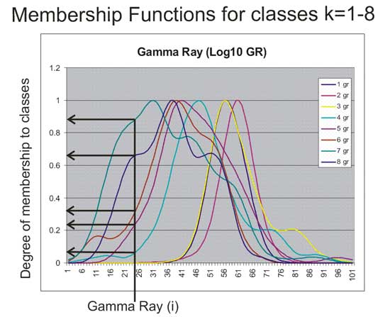
For each observation (i) the degree of membership (DM) for each feature element (j) to the membership function for each class (k) was determined by linear interpolation between points in the membership function (jk). For data including the PE, input is a seven-unit feature vector and output has 56 elements, eight values for the degree of membership to each class for each input value. Where PE is not available the DM is zero for that element in the output vectors. The output vectors for a 3D array (ijk) where i is the DM for variable j in class k. Figure 7 shows schematically the FzLC used in this study.
Figure 7--Fuzzy logic schematic.
The fuzzy decision module chosen for this exercise is a simple one. The degree of membership values in each output vector were summed by class, reducing the vector to 2D (1X8), and the predicted class was determined to be the one with the maximum summed DM. This is a simple but very logical approach since the degree of belongingness to a class would, by intuition, be a function of the summed DM of that observation to the membership functions associated with that class. One slight variation introduced was weighting of the DM by variable. That is, some of the variables were weighted by multiplying the associated DM by a constant, discussed later.
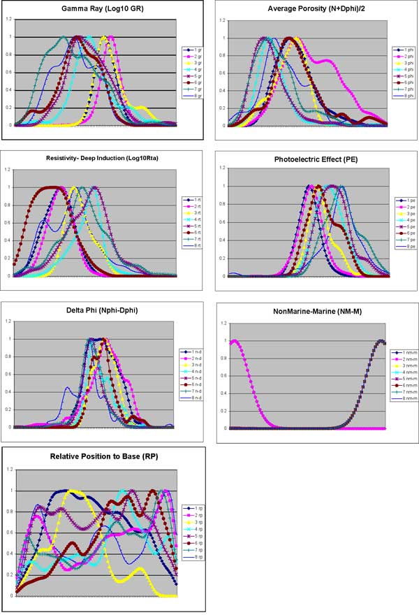
Possibly the most critical part of developing the FzLC is defining the feature space associated with each variable for each class (Figure 8). The advantage of fuzzy logic over more traditional classifiers (e.g.: Bayes and other discriminant analysis) is that in problems where the variable space is irregular, overlapping, and generally fuzzy, the space can be defined with a high degree of precision, provided there is sufficient data. There does appear to be sufficient data to accurately define this space in this problem.
Figure 8--Membership Functions. Class (k=8) membership functions (MF) for the seven variables (j). Thes are for kernal smoothing window dimensions u0 that are fairly close to the optimized u. The MF space is divided by 100 and the values at each point on the y-axis (the observation value) is stored in a 1 x 101 array. A larger version of this figure is available.
There are only two parameters to optimize in this FzLC, smoothing window (u) in the ksdensity function and the weights to be applied to the DM by variable (j). Statistics of the membership functions generated by ksdensity function using the default smoothing window width (u) were compared with actual data statistics to determine whether the synthetic membership functions were satisfactory. The default u is approximately 0.04 of the range of the data appeared too smooth and a series of other u as a function of range were tested. The smoothing window was further optimized by trial and error to those given in Table 5. Initially all weights were either set at 1 (no weighting) and then a second set of weights (wt1) were used in a second run. The weights were later optimized along with u by trial and error using % correct classification as a metric. Final weights and u are also shown in Table 5.
Table 5--Evolution of parameter optimization.
The training of the FzLC is essentially developing the membership functions from the training data. The same training and test sets used in the Bayesian Classifier were used here, but there need not be two training sets (one with PE and one without PE). Due to the structure of the classifier both those data using the PE and not using the PE can be used in training simultaneously. Once "trained" both the training pattern (2/3rd of the data) and the test pattern (1/3rd of the data) were classified by the FzLC program and output was analyzed in Excel. Results in are shown in Table 6 and Figures 9 and 10.
Table 6--Summary table: classification success metrics, Fuzzy logic.
| Train | Test | ||||||
|---|---|---|---|---|---|---|---|
| opt u&wt mixed |
opt u&wt PE exmpls |
opt u&wt PE not used |
opt u&wt mixed |
opt u&wt PE exmpls |
opt u&wt PE not used |
u1w1 mixed |
|
| Correct | 0.64 | 0.65 | 0.63 | 0.61 | 0.62 | 0.60 | 0.59 |
| Close (±1F) | 0.91 | 0.92 | 0.90 | 0.89 | 0.89 | 0.88 | 0.88 |
| F678Correct | 0.50 | 0.52 | 0.48 | 0.50 | 0.49 | 0.49 | 0.46 |
| 678Close ±1F | 0.94 | 0.95 | 0.93 | 0.90 | 0.92 | 0.90 | 0.89 |
| F678 %Actual | 1.04 | 1.08 | 1.07 | 1.15 | 1.14 | 1.21 | 1.10 |
| SD %Actual (all) | .059 | 0.58 | 0.61 | 0.51 | 0.53 | 0.56 | 0.55 |
Figure 9--Plot of fuzzy logic metrics
Figure 10--Fuzzy logic pivot tables compare predicted facies with actual. Numbers on the diagonal are those examples that were predicted correctly.
Three types of tests were run on both the training and test sets: (1) mixed, using seven variables when PE is not available and six when not, (2) PE examples alone, where PE was available, a subset of 1, and, (3) PE not used, but run on the entire set. Optimized parameters u and wt were used for the six runs. The seventh example is of the "mixed" variety using u1wt1, essentially the default u and wt. Some general comments may be made about the results (Table 6 and Figure 9):
Pivot tables in Figure 10 provide a look inside the statistics in Table 6 and Figure 9 for two of the runs, class predictions for the test sets for the mixed and PE only sets. It is readily evident that this FzLC does not do a very good job of classifying some facies (classes), in particular classes 4, 6 and 8. Class 4 is significantly under represented at only 12% and 14% of actual predicted while class 6 is significantly over represented at 200% in both runs shown. Class 8 is more closely represented, but the % correct for this class is quite low at 29 and 30%.
A conventional feed-forward back-propagating artificial neural network (ANN) that is a program in Kipling, an Excel add-in developed by Bohling and Doveton at the KGS, was used for most of this portion of the project, instead of Matlab, primarily because of the past related work that had been done on this platform. The neural network tool in Kipling2, the latest version, uses a simple single hidden-layer neural network with k softmax-transformed outputs representing probabilities of membership in k different classes, a categorical prediction. The prediction code is contained entirely within Kipling2, but the neural network function from the R statistical analysis package does the training. R is the open-source version of the statistical computing language S.
The ANN used in this exercise (Figure 11) has either seven (with PE) or six (without PE) input nodes a single hidden layer with variable number of nodes and eight output nodes, one for each class (facies). The output nodes are probabilities for a given class (facies). Weights are randomly initialized and adjusted in the backpropogating-feedforward training exercise with the cross-entropy objective function being the metric for training. Parameters that were optimized in earlier work by Bohling (Dubois etal, 2003a,b, Bohling, 2003) include the number of iterations the ANN is allowed (100), number of hidden layers (50), and the damping parameter (0.1). The damping parameter constrains the magnitude of the network weights to help prevent overtraining.
Figure 11--Schematic of the ANN used in this project.
The training and testing data was handled in a similar manner as with the earlier classifiers, however, consideration was given to equalizing the data so that all classes were equally represented. It was felt that unequal class sizes could lead to the ANN being overly trained and biased in favor of the larger classes. Test results comparing ANN's trained on data sets having equal class sizes compared to one with unequal class size are shown in Table 7. Equalization may provide minimal prediction improvement in some metrics but not in others. Training ANN's on unequal class sizes does not appear to have significant impact on the classification effectiveness and the training sets were not equalized in this project.
Table 7--Test results of artificial neural network.
| Equal1 | Equal2 | Equal3 | Not Equal Complete |
|
|---|---|---|---|---|
| Correct | 65.3% | 65.2% | 63.7% | 68.8% |
| Close (±1F) | 89.1% | 90.5% | 89.1% | 93.9% |
| F6-8 Correct | 60.6% | 60.6% | 59.0% | 52.7% |
| F6-8 Close | 84.2% | 88.3% | 85.3% | 90.0% |
| F6-8 %Actual | 97.6% | 100.8% | 97.8% | 96.3% |
| SD %Actual | 11.7% | 9.6% | 8.1% | 14.4% |
The input variables GR and Rta have very large ranges in the data set and the data are normally distributed and it was thought that using the Log10 of the values rather than actual measured values might give better results. Both types of data were tested and the results (Table 8) indicate using Log10 of the values had little impact on the prediction success. The differences between the test sets are likely within the range of variability inherent in the different ANNs due to randomization of initial weights.
Four ANN's were trained, two using Log10 data, NoPE and PE, and two using original, untransformed data, NoPE and PE. Each of the four ANN's was then simulated on two sets of data, the training set (2/3rd) and the withheld test set (1/3rd). The "NoPE" set included all examples from the test set and the "PE" data included those data that had a PE curve available. As indicated earlier, there are eight output nodes representing the probability of membership to all of the eight classes. For this project, these were converted to a crisp output using a "winner-take-all" approach. Results of the classification exercise are shown Figure 12 and Table 8.
Table 8--Summary table: classification success metrics, conventional ANNs.
| Log10 Rt and GR | Original (no log) | |||||||
|---|---|---|---|---|---|---|---|---|
| Train PE |
Train NoPE |
Test PE |
Test NoPE |
Train PE |
Train NoPE |
Test PE |
Test NoPE |
|
| Correct | 0.89 | 0.77 | 0.78 | 0.68 | 0.86 | 0.78 | 0.75 | 0.67 |
| Close (±1F) | 0.98 | 0.95 | 0.94 | 0.93 | 0.97 | 0.96 | 0.93 | 0.93 |
| F6-8 Correct | 0.82 | 0.68 | 0.66 | 0.53 | 0.81 | 0.63 | 0.57 | 0.50 |
| F6-8 Close (±1F) | 0.96 | 0.92 | 0.86 | 0.87 | 0.95 | 0.90 | 0.82 | 0.83 |
| F6-8 %Actual | 0.93 | 0.93 | 1.00 | 1.04 | .095 | 0.95 | 0.92 | 0.97 |
| SD %Actual (all) | 0.08 | 0.17 | 0.21 | 0.19 | 0.09 | 0.19 | 0.18 | 0.20 |
Figure 12--Plot of classification success metrics.
The six metrics do not vary significantly when comparing a single simulation run with another. However, some persistent parallel trends suggest the data are real and not merely a reflection of the natural variability between different ANN realizations.
Considering only runs on the withheld test data, the following can be said:
In general, the ANN does a fairly good job of facies prediction if the required accuracy is within one class or facies. The PE curve does help significantly on the absolute accuracy metric, but not having a PE curve is not deleterious when considering the "close" metric. The Facies proportions predicted are fairly good overall. Pivot tables in Figure 13 provide a look inside the statistics in Figure 12 and Table 8. Facies 4 and 8 continue to be difficult to accurately predict with many of 4 being predicted as 5 and facies 8 are often predicted as facies 7.
Figure 13--ANN classifier pivot tables compare predicted facies with actual. Numbers on the diagonal are those examples that were predicted correctly.
Analyzing the results and discussion of the three classifiers should be done within the context of the objectives of the classification exercise. The metrics chosen for determining the success of a classifier were designed with the objectives in mind. Absolute correctness is important and desirable, however, considering the fuzzy nature of the facies and the inherent error in the data, being close (within one facies) is nearly as important as being precise. Having a facies model that approximates the relative proportions and distribution of facies is another objective.
1. Figure 14 illustrates that all three classifiers are fairly close on the absolute correctness metric, though a slight edge goes to the ANN's, especially when considering all facies. The margin is less when considering F678.
Figure 14--Correct classifications for 3 classifiers.
2. Figure 15 shows a comparison of the three classifiers using the closeness metric (percent correct within 1 facies). When considered alone this metric would indicate the success of the three classifiers are about equal. The ANN's are actually lower in the closeness metric when it comes to the key facies 6-8.
Figure 15--Correct class within one class.
3. Figure 16 shows the metrics related to the ratio of number of predicted to actual facies by class. The ANN clearly does a much better job than the other two classifiers with very close to 100% for that metric while the others are over predicting substantially. The second metric in the figure shows the overall balance in the predicted facies through the standard deviation of the predicted/actual by class. Low standard deviation indicates less variance, which is good. Here, the ANN's are the clear winners.
Figure 16--Ratio of predicted to actual and the standard deviation, by class.
The metrics in Figure 16, coupled with the pivot tables throughout the earlier discussions, shed considerable light on the metrics in Figures 14 and 15. The reason for the successful classifications for facies 6-8 for the Bayes and fuzzy classifiers is due, in a large part, to over prediction of those facies. The variance in the ratios of predicted/actual may indicate a high level of instability in those classifiers, while the relatively low variance between classes in the ANN tends to indicate it is doing a fairly good job of at least getting close in most instances.
Of the three classifiers designed and tested in this rock facies classification problem the ANN far outperformed both the fuzzy logic classifier and the Bayesian classifier. Considering the nature of the data and the objectives, the ANN may be an adequate tool for assisting in the identification of rock facies in the Panoma Field in southwest Kansas. The ANN does have some shortcomings, especially in correctly classifying facies 4 and facies 8, that deserve further work. Perhaps combining fuzzy logic and the neural network could provide some improvement, although fuzzy logic also had problems in facies 4 and facies 8. A very simple decision module for the fuzzy logic model was used, and additional work is needed to develop a more robust rules-based operator and decision module for this classifier before it is eliminated from consideration. It does appear that traditional discriminant analysis methods like Bayes are ineffective. The results of experiments discussed in this report support the basic concept of using automated statistics based tool for facies classification, but it also shows that there are limits to effectiveness with this particular data set.
Dubois, M.K., Byrnes, A.P., Bohling, G.C., Seals, S.C., and Doveton, J.H., 2003a, Statistically-based lithofacies predictions for 3-D reservoir modeling: an example from the Panoma (Council Grove) Field, Hugoton Embayment, southwest Kansas, (abs.): American Assoc. of Petroleum Geologists, 2003 Annual Convention, vol. 12, p. A44; also in Kansas Geological Survey, Open-file Rept. 2003-30. [available online]
Dubois, M.K., G.C. Bohling, A.P. Byrnes, and S.C. Seals, 2003b, Extracting Lithofacies from Digital Well Logs Using Artificial Intelligence, Panoma (Council Grove) Field, Hugoton Embayment, Southwest Kansas, (abs.): American Assoc. of Petroleum Resources, Mid-continent Section Meeting, Tulsa; also in Kansas Geological Survey, Open-file Rept. 2003-68. [available online]Saggaf, M.M. and E.L. Nebrija, 2003, A fuzzy logic approach for the estimation of facies from wire-line logs: American Assoc. of Petroleum Resources, Bulletin, v. 87, no. 7, p. 1223-1240.
Kansas Geological Survey, Energy Research
Placed online May 6, 2005
Comments to webadmin@kgs.ku.edu
The URL for this page is HTTP://www.kgs.ku.edu/PRS/publication/2004/OFR04_64/index.html