Kansas Geological Survey, Open-file Report 2007-25
1 Kansas Geological Survey
2 Agricultural Research Service, USDA
3 Servi-Tech Agri/Environmental Consulting Services
4 Kansas State University, Garden City Experiment Station

Second-year Progress Report to KWRI (March 1, 2006-February 28, 2007)
Kansas Geological Survey, Open-File Report 2007-25
This report is available as an Acrobat PDF file (9.7 MB).
June 2007
1. Problem and Research Objectives
2.1 Field Monitoring/Field Experiments
2.2 Numerical Model Employed
2.3 Outline of Some Model Input Requirements
2.4 Model Calibration Procedures
2.4a General Procedures
2.4b Sensitivity Analysis
2.4c Calibration Strategy
3.1 Soil Nitrate ProfIles
3.2 Wastewater and Ground-water Quality
3.3 Dye-tracer Experiment Results
3.4 Sensitivity Analysis Results
3.5 Model Calibration and Simulation Results
3.6 Management Scenarios Results
4. Publications and Presentations
With increasingly limited ground-water resources, reuse of treated wastewater provides an alternative source of water for irrigation of crops and landscaping. In addition, utilization of the nutrients in recycled wastewater as fertilizer results in less application of fertilizer to a plant system.
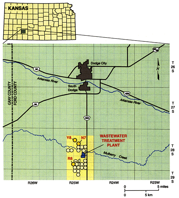
A long-term irrigation project using treated municipal wastewater has been ongoing south of Dodge City in Ford County since the mid-1980s (Fig. 1). The Dodge City Wastewater Treatment Plant (DCWTP) consists of three covered anaerobic digesters and three aeration basins. The treated water is stored in storage lagoons with a capacity of more than 2800 acre-ft. A pumping system, consisting of several electric, centrifugal pumps distributes the water to irrigate more than 2700 acres of cropland in 25 fields (Fig. 1). The system is managed by Operations Management International (OMI) and the agronomic firm Servi-Tech, Inc., under contracts with the City.
Figure 1--Location of the study area. Circular areas indicate irrigated fields.
Use of the treated wastewater, which includes inputs from both the municipality of Dodge City and its meat-packing plant, has resulted in relatively high soil nitrate-nitrogen concentrations (10-50 mg/kg) in the soil profile at the sites irrigated with this treated wastewater effluent as well as in nitrate-nitrogen concentrations in ground water from monitoring wells in the area exceeding the safe drinking-water limit of 10 mg/L (Zupancic and Vocasek, 2002). Evaluation of the environmental impact of such land-use strategies needs to be made in order to determine if and when this process may impact usable ground water at depth and what management changes may need to be made to slow the downwards nitrogen (N) migration.
The study area overlies the High Plains aquifer with depth to water in the range of 75 to 150 ft. The overlying soils are predominantly Harney and Ulysses silt loams (Dodge et al., 1965). Although this area has a deep water table and soils with a silty clay component, there is evidence that nitrate is migrating to those depths through the vadose zone. USGS National Water-Quality Assessment and other studies in the central High Plains aquifer region indicate that nitrate from fertilizer sources and animal waste has reached the Ogallala portion of the High Plains aquifer most likely due to increased recharge from irrigation but also because of preferential flow processes (U.S. Geological Survey, 2004).
It is now generally recognized that preferential flow occurs to some degree in most soils (Shipitalo and Edwards, 1996). In some soils, macropores can serve as important pathways for preferential flow that allow rapid gravitational flow of the free water available at the soil surface or above an impeding soil horizon, thus bypassing the soil matrix. Short-circuiting to ground water through macropores is of serious concern because of the possibilities of rapid transport of a portion of fertilizers, pesticides, and other chemicals applied on the soil surface. As macropore development, preservation, and continuity can be strongly affected by soil management, such concerns have been exacerbated by the growing practice of minimum or no tillage, which (1) allows chemical solutes in surface water applied on the soil to accumulate and to enter macropores at the surface, and (2) leaves plant residues on the surface as well as no tillage also enhancing worm activity and allowing worm holes and other macropore channels to stay open at the surface (Ahuja et al., 1993).
Therefore, the objectives of this project are
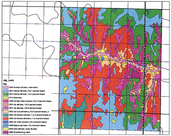
To analyze this nitrogen-leaching problem further, we established two main monitoring sites, one in each of the two major loess-derived soil series in the project area, the Harney and the Ulysses soils (Fig. 2; the Harney silt loams are the bluish and greenish colors in the slide, whereas the Ulysses silt loams are the reddish and purplish colors). One of the sites, the R8 in Harney soils, has a long-term treated wastewater irrigation history (since 1986), whereas the other site, N7 in Ulysses soils, has a short-term treated wastewater irrigation history (since 1998). In addition, a third, control site, Y8, without any wastewater irrigation record, has also been established (Fig. 2). Crop-history records indicate that corn (Zea mays L.) was planted at site N7 each year since 1998, and at site R8 since 2003. From 1997 to 2002, site R8 was planted in alfalfa (Medicago sativa). During 2005, sites N7 and R8 were planted in corn, whereas site Y8 was planted in sorghum (milo). During 2006, all three sites were planted in corn.
Figure 2--Map of soils in Ford County at study sites (data downloaded from the NRCS Geospatial Data Gateway at http://datagateway.nrcs.usda.gov/).
We collected several deep cores, down to 15.2 m, from each of the sites for a number of physical and chemical analyses using a truck-mounted Giddings probe. The textural, soil hydraulic, and additional physical and chemical analyses were performed by NRCS personnel at the Lincoln, NE, National Soils Laboratory. Core nitrogen and carbon and related analyses were conducted at the KSU and Servi-Tech Soil Analysis Laboratories. Tables and figures of analyzed values are presented in Sophocleous et al. (2006) and are summarized by model simulation layer in section 2.3.
The soil bulk density down to 15.2 m was determined from collected cores of known diameter by cutting the core in 15.2-cm (6-inch) increments, weighing them in the field, and then oven-drying them in the lab. For a smoother bulk density profile estimation, a three-consecutive 15.2-cm core-sample moving average was obtained down to 15.2 m.
A neutron probe (Campbell Pacific Nuclear (CPN) 503DR Hydroprobe) is used to collect moisture-data profiles to 15.2-m depth. Aluminized steel pipe was used for the neutron probe access tube. The neutron probe was calibrated in the field as follows: a 15.2-m hole was cored with the Giddings probe, and the access tube was snuggly inserted down the hole. The collected core was cut in 15.2-cm increments, weighed in the field, and taken to the Servi-Tech, Inc., soils lab for oven-drying and re-weighing. Following access-tube installation, neutron profile readings were taken in 15.2-cm increments within the root zone (180 cm) and in 30.48-cm increments from the bottom of the root zone to 15.2 m. At each site, two field corner (180- by 180-cm) plots were selected as additional calibration plots in which a 305-cm access was installed in each. One plot was used for the neutron-moisture calibration at the dry end-end of the moisture range, whereas the other plot was periodically wetted by applying measured amounts of water for neutron probe calibration at the wet end of the moisture range. Periodically, 244-cm-long cores were collected from within the corner, calibration plots were done with the Giddings probe, and moisture content was calculated by oven-drying for comparison with neutron readings. Additional details of neutron access tube installation and probe calibration are presented in Sophocleous et al. (2006). Periodic measurements of neutron probe-based soil water content down to 15.2 m were conducted throughout the growing seasons for 2005 and 2006.
A small number of suction lysimeters were also installed in all sites at various depths, mainly at shallow (152-183 cm) and intermediate depths (518-793 cm) for occasional analyses of pore waters.
We also sampled most of the existing monitoring wells in the area (shown in Fig. 9) to check any impacts on the relatively deep water table, which ranges from about 21 m close to Mulberry Creek to more than 45 m deep as one goes away from the usually dry Mulberry Creek (Fig. 1). Additional water samples from monitoring, domestic, and irrigation wells and wastewater lagoons were periodically collected by OMI and occasionally KGS personnel.
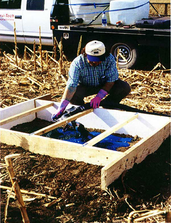
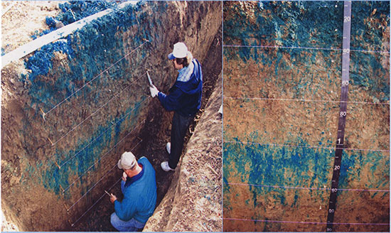
To explain deep occurrences of nitrogen concentrations through possible preferential pathways, we conducted two dye-tracer experiments in each of the two major soil types in the study area in which we established our study sites (site R8 in Harney soil, and site N7 in Ulysses soil). A literature search for a suitable dye tracer (Flury and Fluhler, 1994, 1995; Flury et al., 1994; Petersen et al., 1997; Schwartz et al., 1999; Flury and Wai, 2003) revealed that the brilliant-blue food-coloring dye (FD&C Blue 1, triphenyl-methane dye) would be a suitable tracer because of its desirable properties of mobility and distinguishability in soils, and also because of its non-toxicity.
The steps we followed in conducting the dye-tracer tests at sites R8 and N7 are as follows: we rented a 3785-liter (1000-gallon) water tank and filled it with 1514 liters (400 gallons) of water. We then added a carefully pre-weighted total quantity of 6,056.7 grams of brilliant-blue powder dye (3,028.4 grams per 757 liters {200 gallons} of water) and mixed it well to obtain a dye concentration of 4 g/L (which was also employed in the studies cited above). We prepared two 91.4-cm by 152.4-cm (3-ft by 5-ft) wooden rectangular frames of 91.4-cm height for flooding the sites with the dye solution as shown in Figure 3.
Figure 3--Wooden rectangular frame for flooding the site with dye solution.
The USDA-ARS developed a Root Zone Water Quality Model (RZWQM), which is a comprehensive agricultural systems model intended as a research tool to investigate the effects of agricultural management on crop production and environmental quality (Ahuja et al., 2000). The RZWQM is an integrated physical, biological, and chemical process model that simulates plant growth, and the movement and interactions of water, nutrients, and pesticides over and through the root zone at a representative area of an agricultural cropping system. It is a one-dimensional (vertical into the soil profile) model designed to simulate conditions on a unit-area basis.
The reasons we chose to evaluate the RZWQM model are because, in addition to having been extensively tested nationally and internationally (Ahuja et al., 2000; Abrahamson et al., 2005; Malone et al., in press), it contains special features of interest to this study, such as macropore flow as well as an exchange component between the soil matrix and macropore walls; a wide variety of management effects, such as evaluation of conservation tillage, residue cover and conventional tillage, methods and timing of water applications as well as fertilizer and pesticide applications, and different crop rotations; and a user-friendly interface that can be initially set up with a minimum dataset using readily available data, as well as other features.
The RZWQM consists of six subsystems or processes that define the simulation program: 1) physical processes 2) soil chemical processes 3) nutrient processes 4) pesticides processes 5) plant growth processes and 6) management processes. Information about the RZWQM processes is calculated at daily and sub-hourly time scales as shown in Figure 4.
Figure 4--Execution sequence for RZWQM (adapted from Ahuja et al., 2000).
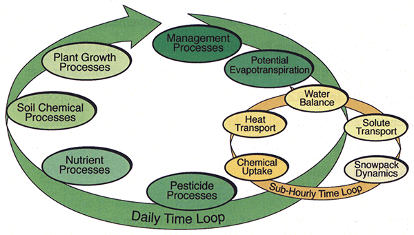
Management effects on the system (such as tillage, addition of chemicals or irrigation water) are calculated first. A daily estimate of potential ET is then determined (based on an extended Shuttleworth-Wallace potential ET module (Farahani and Ahuja, 1996) that considers the effects of surface-crop residue cover on soil evaporation and partitions evaporation into the bare soil and residue-covered fractions) so that the evaporation and transpiration fluxes can be applied to the soil surface and plant roots, respectively.
The sub-hourly time loop is then executed to calculate the transport and fate of the water-controlled processes. These processes include infiltration and runoff, soil water distribution, chemical transport, actual evaporation and transpiration, plant nitrogen uptake, and others.
The water flow processes in the RZWQM are divided into two phases: 1) infiltration into the soil matrix and macropores and macropore-matrix interaction during a rainfall or an irrigation event, modeled by using the Green and Ampt approach; and 2) redistribution of water in the soil matrix following infiltration, estimated by a mass-conservative numerical solution of the Richards' equation. Rainfall or irrigation water in excess of the soil-infiltration capacity (overland flow) is routed into macropores if present. The maximum macropore flow rate and lateral water movement into macropores in the surrounding soil are computed using Poiseuilles' law and the lateral Green-Ampt equation, respectively. Macropore flow in excess of its maximum flow rate or excess infiltration is routed to runoff. In the RZWQM, water can only enter the macropores at the surface. High-intensity rainfalls generally yield greater water flow and chemical transport in macropores than low-intensity rainfalls (Shipitalo and Edwards, 1996), and this is true with the RZWQM as well.
Continuing along the daily loop, pools of carbon and nitrogen are transformed by the nutrient processes (Ma et al., 1998). The soil carbon/nitrogen dynamics module of the RZWQM model (Hanson et al., 1999) contains two surface residue pools (fast and slow decomposition), three soil humus pools (slow, medium, and fast decomposition), and three soil microbial pools (aerobic heterotrophs, autotrophs, and anaerobic heterotrophs). It simulates N mineralization, nitrification, denitnification, ammonia volatilization, urea hydrolysis, methane production, and microbial population. These processes are functions of soil pH, soil O2, soil microbial population, soil temperature, soil water content, and soil ion strength. Despite the complexity of this organic matter/N-cycling component, good estimates of initial soil carbon content and nitrogen are generally the only site-specific parameters needed. The required inputs (e.g. fast pool, slow pool) are then usually determined through an initiation wizard and calibration.
Finally, after accounting for all the physical and chemical changes to the system throughout the day, the plant-growth processes determine crop production. The RZWQM has a generic plant-growth component that can be parameterized to simulates different crops. Both individual plant growth through seven phenological growth stages (dormancy, germination, emergence, 4-leaf plant, vegetative growth, reproductive growth, and senescence), and population development (controlled by the Leslie matrix {Hanson, 2000}) are simulated. The RZWQM also provides a second option submodel for simulation of crop growth referred to as the Quickplant model. However, Quickplant is not a detailed growth model, and it is recommended (Ahuja et al., 2000) that it only be used when simulating crop production is not a primary aim of the modeler. Details on all aspects of the model can be found in Ahuja et al. (2000).
As mentioned previously, the RZWQM is a research-grade complex tool that was designed to analyze soil and plant processes only within the root zone. However, for our application, we had to modify and extend the RZWQM to deal with deeper vadose-zone processes, and in discussing this extension with the RZWQM developers in the Agricultural Research Service Systems-Research Unit in Fort Collins, CO, ours may be the first RZQWM application to depths beyond the root zone. Soil-horizon depths are converted to a numerical grid with a maximum thickness of 5 cm and 1 cm for the top soil layer. These numerical layers are used for solving the Richards equation during redistribution. During infiltration, 1-cm soil layers are used for the Green-Ampt equation (Ahuja et al., 2000). This model can simulate a soil profile of up to 30 m. A unit gradient was assumed for the lower boundary condition at 10.8 m for site N7 and 4.84 m for site R8.
To simulate the transport of water and chemicals, the soil profile must be well defined in its depth, horizon delineation, physical properties (bulk density, particle density, porosity, and texture), and hydraulic properties. A detailed description of site soil horizons and related physical and chemical properties is presented in Sophocleous et al. (2006). Because of model limitations, we had to combine a number of soil horizons into a maximum of 10 layers. The soil physical properties by layer used as initial conditions for model simulations {based on NRCS National Soils Lab (Lincoln, NE)-analyzed soil-core measurements that were presented in Sophoc1eous et al. (2006)} are shown in Tables 1 and 2 for sites N7 and R8, respectively.
Table 1--Soil physical properties for site N7 by layer based on measurements by the NRCS National Soils Lab (Lincoln, NE) that are presented in Sophocleous et al. (2006)
| Layer | Soil Type | Horizon Depth (cm) |
Bulk Density (g/cm3) |
Porositya | Sand fraction |
Silt fraction |
Clay fraction |
Ksb (cm/hr) |
1/3-bar W.C.c |
1/10-bar W.C.c |
15-bar W.C.c |
|---|---|---|---|---|---|---|---|---|---|---|---|
| 1 | Silty loam | 0-23 | 1.280 | 0.517 | 0.056 | 0.686 | 0.258 | 1.3163 | 0.2260 | 0.3637 | 0.1305 |
| 2 | Silty clay loam | 23-74 | 1.470 | 0.445 | 0.027 | 0.621 | 0.352 | 0.3911 | 0.2540 | 0.4037 | 0.1690 |
| 3 | Silty clay loam | 74-168 | 1.300 | 0.509 | 0.033 | 0.624 | 0.343 | 0.7268 | 0.2710 | 0.4037 | 0.1617 |
| 4 | Silty clay loam | 168-221 | 1.240 | 0.532 | 0.114 | 0.558 | 0.328 | 0.9829 | 0.2390 | 0.4037 | 0.1410 |
| 5 | Silty clay loam | 221-363 | 1.380 | 0.479 | 0.115 | 0.554 | 0.331 | 0.2266 | 0.2070 | 0.3742 | 0.1215 |
| 6 | Silty clay loam | 363-625 | 1.420 | 0.464 | 0.090 | 0.610 | 0.300 | 0.5431 | 0.2340 | 0.4037 | 0.1185 |
| 7 | Silty loam | 625-848 | 1.350 | 0.491 | 0.126 | 0.631 | 0.243 | 0.7048 | 0.2855 | 0.3637 | 0.1070 |
| 8 | Silty loam | 848-889 | 1.380 | 0.479 | 0.141 | 0.638 | 0.221 | 0.6966 | 0.2855 | 0.3637 | 0.1260 |
| 9 | Silty loam | 889-945 | 1.410 | 0.468 | 0.267 | 0.513 | 0.220 | 0.6966 | 0.2480 | 0.2961 | 0.0960 |
| 10 | Loam | 945-1079 | 1.520 | 0.426 | 0.344 | 0.416 | 0.240 | 0.1463 | 0.2335 | 0.2961 | 0.1015 |
| a calculated assuming a particle density of 2.65 g/cm3 b saturated hydraulic conductivity (Ks) c soil water content (W.C.) |
|||||||||||
Table 2--Soil physical properties for site R8 by layer based on measurements by the NRCS National Soils Lab (Lincoln, NE) that are presented in Sophocleous et al. (2006)
| Layer | Soil Type | Horizon Depth (cm) |
Bulk Density (g/cm3) |
Porositya | Sand fraction |
Silt fraction |
Clay fraction |
Ksb (cm/hr) |
1/3-bar W.C.c |
1/10-bar W.C.c |
15-bar W.C.c |
|---|---|---|---|---|---|---|---|---|---|---|---|
| 1 | Silty clay loam | 0-16 | 1.420 | 0.464 | 0.041 | 0.643 | 0.316 | 0.4480 | 0.4463 | 0.4037 | 0.2107 |
| 2 | Silty clay loam | 16-29 | 1.490 | 0.438 | 0.036 | 0.659 | 0.305 | 0.4452 | 0.4216 | 0.4037 | 0.2107 |
| 3 | Silty clay loam | 29-50 | 1.280 | 0.517 | 0.023 | 0.599 | 0.378 | 0.1553 | 0.4928 | 0.4037 | 0.2107 |
| 4 | Silty clay | 50-68 | 1.210 | 0.543 | 0.017 | 0.553 | 0.430 | 0.0890 | 0.5182 | 0.4251 | 0.2513 |
| 5 | Silty clay loam | 68-90 | 1.260 | 0.525 | 0.021 | 0.592 | 0.387 | 0.2799 | 0.5002 | 0.4037 | 0.2107 |
| 6 | Silty clay loam | 90-140 | 1.520 | 0.426 | 0.030 | 0.627 | 0.343 | 0.8501 | 0.4280 | 0.4037 | 0.2107 |
| 7 | Silty clay loam | 140-260 | 1.620 | 0.389 | 0.152 | 0.502 | 0.346 | 0.3237 | 0.4049 | 0.3890 | 0.2107 |
| 8 | Silty clay loam | 260-300 | 1.610 | 0.392 | 0.194 | 0.483 | 0.323 | 0.1543 | 0.3806 | 0.3920 | 0.2107 |
| 9 | Clay loam | 300-410 | 1.530 | 0.423 | 0.217 | 0.494 | 0.289 | 0.2968 | 0.4230 | 0.3742 | 0.1882 |
| 10 | Silty clay loam | 410-484 | 1.540 | 0.419 | 0.188 | 0.496 | 0.316 | 0.1308 | 0.4380 | 0.4037 | 0.2107 |
| a calculated assuming a particle density of 2.65 g/cm3 b saturated hydraulic conductivity (Ks) c soil water content (W.C.) |
|||||||||||
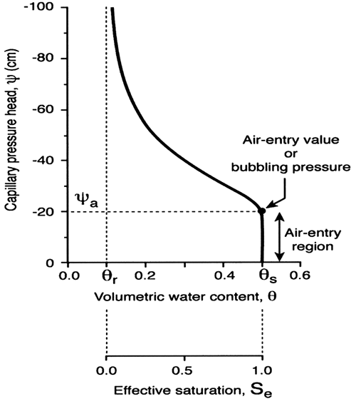
The hydraulic properties are defined by the soil water characteristic or retention curves, and the unsaturated hydraulic conductivity function. Those relationships are described by functional forms suggested by Brooks and Corey (1964) with slight modifications (Ahuja et al., 2000).
The volumetric soil water content (θ) versus the capillary pressure head or matric suction head (ψ) relationship representing the water retention or characteristic curve is formulated as follows:
θ (ψ) = θs - A1|ψ| for ψ ≤ ψa (1)
θ (ψ) = θr + B|ψ|-λ for ψ > ψa (2)
where θs and θr are the saturated and residual soil-water contents (cm3/cm3), respectively; ψa is the air-entry or bubbling suction head (cm); λ is the pore-size distribution index (and represents the logarithmic slope of the water retention curve); A1 and B are constants, where B = (θs - θr - A1ψa)ψaλ and A1 was set to zero in our case, thus reducing equations (1) and (2) to the Brooks and Corey (1964) model. Figure 5 displays a schematic of a typical soil-water retention curve with a number of the above-mentioned parameters indicated.
Figure 5--Schematic of a typical soil-water retention curve.
The hydraulic conductivity (K) versus matric suction head (ψ) relationship representing the unsaturated hydraulic conductivity function is formulated as follows:
K(ψ) = Ks|ψ|-N1 for ψ ≤ ψa (3)
K(ψ) = K2|ψ|-N2 for ψ > ψa (4)
where N1, N2, and K2 are constants and K2 = Ks = |ψa|-N2, N2 = 2 + 3λ, and N1 was set to zero in our case, thus reducing equations (3) and (4) to the Brooks and Corey (1964) model, where the effective saturation, S, is defined as Se = (θ - θr) / (θs - θr)
The RETention Curve (RETC) computer program (van Genuchten et al., 1991) for describing the hydraulic properties of soils as well as the neural network program ROSETTA (Schaap et al., 2001) were employed to fit the parameters for several analytical models such as the Brooks and Corey (1964) and van Genuchten functions (van Genuchten, 1980) to experimentally measure water retention and hydraulic conductivity data for input into the RZWQM. (The correspondence of the van Genuchten parameters α and n to the Brooks and Corey parameters ψa and λ is as follows: α = 1/ψa, and n = λ + 1.)
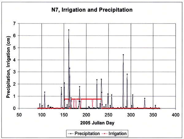
The model also requires detailed meteorological data on a daily basis, and rainfall data in breakpoint increments. Hourly precipitation and other meteorological data (except for solar radiation) were obtained from the Dodge City Municipal Airport weather station, some 17 km northeast of the study sites, whereas daily solar radiation data were obtained from the Garden City Agricultural Experiment Station some 80 km west-northwest of Dodge City, operated by Kansas State University. The model also requires specification of land-use practices such as planting and harvesting dates, specification of irrigation and fertilization events, as well as the chemical quality of irrigation. The daily precipitation and irrigation events during the 2005 irrigation season for site N7 are shown in Figure 6.
Figure 6--Daily precipitation and irrigation events during the 2005 irrigation season at site N7.
The physically based nature of RZWQM necessitates a good deal of data from the user to adequately parameterize and initialize the model. From experience, users do not have enough data to completely describe the state of an agricultural cropping system. To facilitate use of the model, the RZWQM allows for input options where certain parameters are estimated from easily determined soil properties (e.g., soil texture) or obtained from default value tables if measured data are not available.
For accurate simulations, RZWQM must be calibrated for soil hydraulic properties, nutrient properties, and plant-growth parameters for the site and crops being simulated (Hanson et. al., 1999), as there are significant interactions among the different model components. The number of parameters and processes in the RZWQM are so numerous that it is exceedingly difficult to decide which ones to optimize and what optimization scheme might be appropriate, if at all feasible. As a result, such agricultural system models as the RZWQM are usually parameterized by trial-and-error or iterative processes (Ahuja and Ma, 2002). In this report, we followed the detailed procedures for calibrating the RZWQM as laid out by Hanson et al. (1999) and Ahuja and Ma (2002).
The model requires establishment of initial C/N pool sizes for the fast and slow decomposition residue pools; slow, medium, and fast decomposition humus pools; and the three microbial pools (aerobic heterotrophs, autotrophs, and anaerobic heterotrophs) (Hanson et al., 1999). No laboratory procedures are known to effectively determine the sizes of these pools (Ahuja and Ma, 2002). Therefore, because previous management at a site determines the initial state of a soil in terms of its organic matter and microbial populations, simulations with previous management practices will usually create a better initial condition for these parameters (Ma et al., 1998). After entering all the model inputs and parameters, we began by estimating the three humus organic-matter pool sizes (based on measured organic-carbon depth profiles) at 5, 10, and 85%, respectively, for fast, medium, and slow pools and set the microbial pools at 50,000, 500, and 5000 organisms per gram of soil, respectively, for aerobic heterotrophs, autrotrophs, and facultative heterotrophs, as recommended by Ahuja and Ma (2002). RZWQM was initialized for the organic-matter pools by running the model for 12 years prior to the 2005-06 actual simulation periods. A 12-year initialization run was suggested by Ma et al. (1998) to obtain steady-state conditions for the faster soil organic pools. The only parameters that we adjusted after the initialization procedure were the soil nitrate and soil ammonium nitrate for the analysis period (2005-06) as we had available measured values of those quantities from the sites before corn was planted in the spring of 2005.
To identify key model parameters and sources of simulation errors resulting from parameter uncertainty, we conducted extensive sensitivity analysis. A sensitivity analysis is usually done by varying (perturbing) model parameter values around their base values independently. The range of the perturbation may be a specific percentage around a base value (Walker et al., 2000; Ma et al., 2000).
Different sets of model input parameter groups were perturbed, such as 1) hydraulic properties 2) organic matter/nitrogen cycling parameters 3) plant-growth parameters, and 4) irrigation water and fertilization rates. The purpose is to identify key (sensitive) model input parameters under western Kansas conditions in terms of corn production and NO3-N leaching, so as to guide calibration and measurement efforts.
Following the sensitivity analysis, which identified the most sensitive or critical parameters affecting model output, the model calibration strategy we adopted was as follows: the RZWQM was first calibrated for soil hydraulic properties by adjusting one or more of the most sensitive hydraulic parameters from the sensitivity analysis, then for the N-nutrient properties as outlined in the "General Procedures" section, and finally for the plant-growth parameters for the site and crops being simulated. Because plant production was part of the N balance and tightly coupled to the other processes, we followed the procedure for calibrating plant growth recommended for the model by Hanson (2000) when using the generic plant-growth submodel. This procedure is based on adjustments to five relatively sensitive plant parameters (see also section 3.4 on sensitivity analysis results further on for additional explanations) including active N uptake rate (μi), the proportion of daily respiration as a function of photosynthesis (Φ), the specific leaf density, i.e., the biomass to leaf area conversion coefficient (CLA), and the age effect for plants during the propagule stage and the seed-development stage (Ap and As). We based adjustments of these parameters for corn within the range of values used for calibration of the Management Systems Evaluation Areas (MSEA) sites in the midwestern USA (Hanson, 2000). Because the nitrogen-related and plant-growth parameters are difficult to measure with independent experiments, an accurate description of the water-related processes is required to minimize N-simulation errors.
Calibration targets were the measured-profile soil water contents using the neutron probe and the core-sampled nitrate profiles. Field measurement errors are typically &gy; 10%; therefore, it is unrealistic to match the observed data any more closely (Hanson et al., 1999). Both qualitative and quantitative methods were used to evaluate the model. Three statistics were used to evaluate the simulation results: (i) root mean squared error (RMSE) between simulated and observed values, eq. (5); (ii) relative root mean square error (RRMSE), i.e., RMSE relative to the mean of the observed values, eq. (6); and (iii) mean relative error (MRE) or bias, eq. (7).
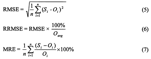
where Si is the ith simulated value, Oi is the ith observed value, Oavg is the average of observed values, and n is the number of data pairs.
The RMSE reflects the magnitude of the mean difference between simulated and experimental results, whereas the RRMSE standardizes the RMSE and expresses it as a percentage that represents the standard variation of the estimator (Abrahamson et al., 2005). The MRE indicates if there is a systematic bias in the simulation. A positive value indicates an overprediction and a negative value an underprediction.
Our coring at the sites indicated relatively high nitrate-N concentrations in the soil profile at all sites sampled as seen in Figure 7 for sites N7, R8, and Y8, respectively. Each curve represents a different soil core analyzed that was collected at the time indicated in the figures.
For site R8 (with a long-term wastewater irrigation history--since 1986) we see (Fig. 7a) a high nitrate peak of about 40 mg/kg around 60 cm, which decreases sharply in the depth interval of 380 to 580 cm, possibly due to previously planted alfalfa roots consuming the nitrate at those depths, as the R8 site was under alfalfa cultivation from 1997 to 2002. The nitrate increases again reaching a secondary maximum near the depth of 880 cm, then following a decrease near the 940-cm level, it progressively increases with depth down to more than 1500 cm. It seems that a previous nitrate front has reached down to 1500 cm, with yet older fronts reaching even deeper, indicating that nitrate may had already penetrated down to those depths.
Figure 7--Measured soil profile Nitrate-Nitrogen during Spring 2005 for all study sites (a - R8, b - N7, and c - Y8), and during Fall 2005 and Spring 2006 for sites R8 and N7.
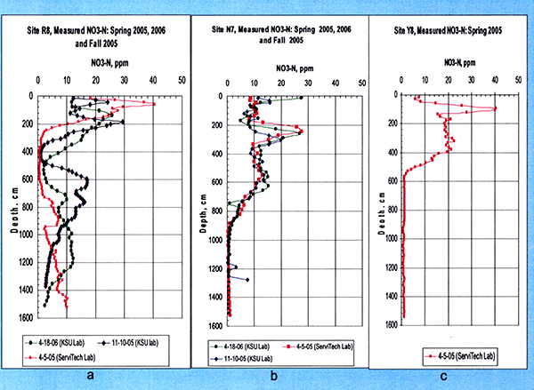
For site N7 (with wastewater irrigation history since 1998) we see (Fig. 7b) a deeper nitrate peak (of less than 28 mg/kg, i.e., not as high as that at site R8) around the 240-cm-depth level. Then, the nitrate distribution progressively decreases to a minimal background level by the time we reach near 900 cm, indicating that nitrate penetrated down to near 900 cm but no further.
Finally, for site Y8 (without any wastewater irrigation), we see (Fig. 7c) a high nitrate peak near the 100-cm level, but by the time we reach the 550-cm depth level, nitrate goes back to minimal background level.
The sites were periodically LEPA-sprinkle irrigated from mid-May until the latter part of August during 2005 and 2006. The general quality of the treated wastewater effluent applied at the sites during 2005 and 2006 is shown in Figure 8. The chloride concentrations (in green) were around the 300 mg/L level but further increased during the second half of the 2006 year, and the Total Kjeldahl Nitrogen concentrations (TKN, in blue) were generally above the 80 mg/L level for site N7. The treated wastewater effluent was analyzed by both the OMI and Servi-Tech labs. The chemical analysis results as analyzed by the OMI lab are presented in Appendix A.
Figure 8--Treated effluent irrigation water chloride, total Kjeldahl nitrogen, and nitrate-nitrogen concentration time series applied to sites N7 (a) and R8 (b) during 2005 and 2006.
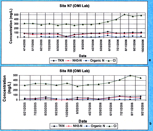
Figure 9 shows the ground-water nitrate-N concentrations from the November 2005 survey sampling, where wells shown in red exceed the safe drinking-water limit for nitrate-N of 10 mg/L. Notice that most of the wells have more than 2 mg/L nitrate-N in the ground water. This indicates (Mueller and Helsel, 1996) that anthropogenic sources have begun to impact the ground water in the area.
Figure 9--Ground-water nitrate-nitrogen concentrations during November 2005. Numbers at the center of square blocks are Section numbers in the Township and Range system of land classification. Green circles/semicircles are irrigated fields.
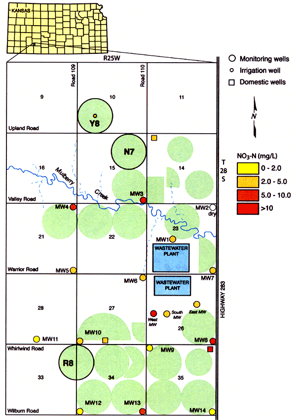
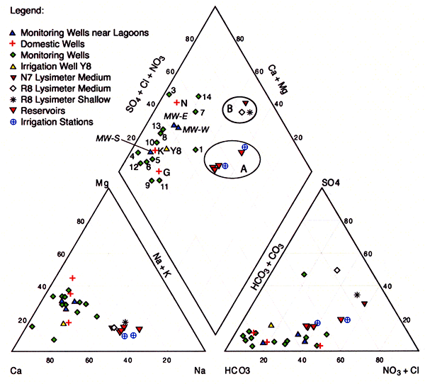
Figure 10 displays a trilinear diagram showing the average water quality of the irrigation water applied in both R8 and N7 sites marked as the A circle, the shallow- and intermediate-depth suction lysimeter-sampled pore water from both sites marked as the B circle, as well as sampled domestic, monitoring, and irrigation wells in the area. The sampled populations of applied wastewater, pore water from suction lysimeters, and monitoring and domestic wells form distinct groups in the trilinear diagram.
Figure 10--Trilinear diagram showing the average 2005 water quality of irrigation water applied in sites R8 and N7 (circle A), the shallow and intermediate-depth suction lysimeter-sampled pore water from sites R8 and N7 (circle B), and the domestic, monitoring, and irrigation wells sampled in the area.
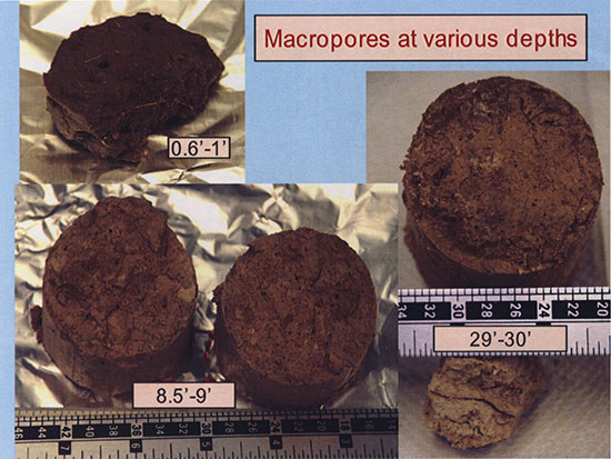
We observed numerous macropores in the cores collected during sampling, not only in the upper soil profile but also at depths down to more than 9 m. Figure 11 displays a small sampling of the observed macropores from the sites. Because of the occurrence of such macropores and of the relatively high nitrate concentrations observed at the various wells sampled in the area, we run the two brilliant-blue dye experiments at the sites that were briefly described in section 2.1.
Figure 11--Soil cores at various depths from the study sites showing macropores. Numbers indicate depth in feet.
For the site R8 in Harney soil, the dye solution penetrated down to approximately 200 cm and formed a more-or-less uniform "finger front" at the bottom as shown in Figure 12. The right-hand-side picture in Figure 12 shows a closer-up view of the dyetracer movement through the blocky-structure soil layers of the Bt horizons (at approximately the 50- to 100-cm depth interval) where the tracer dye moved along the spaces between the blocky soil aggregates and concentrated in numerous fingers in the lower soil layer that did not exhibit the heavy blocky structure of the Bt horizons above.
Figure 12--Uniform finger front from brilliant-blue dye-tracer experiment at site R8. The righthand-side image shows in more detail the dye moving through the inter-soil block structure spaces of the Bt horizon and accumulating below that blocky layer into numerous fingers.
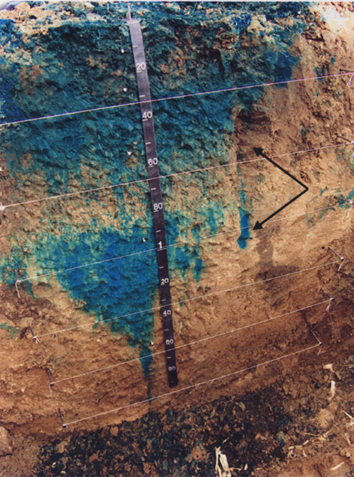
For site N7 in Ulysses soil, the dye pattern was different, forming a giant funnel front ending in a big finger down to approximately 200 cm, as shown in Figure 13. Closer examination of a side finger, indicated in Figure 13, showed that the dye finger formed along a decaying root channel, as did other fingers examined in both sites.
Figure 13--Funnel front pattern from brilliant-blue dye-tracer experiment at site N7 and side finger formed along a decaying root channel (indicated by the two arrows).
The observed macropores at depth are probably due to the existence of deep-rooted prairie grasses that dominated the landscape prior to agricultural development. The currently practiced no-till land-use treatment further enhances worm activity near the soil surface, thus maintaining macropores open at the soil surface. Because of the existence of such preferential-flow pathways, the macropore option of the RZWQM was employed. As a result of the observed macropores throughout the soil profile in both sites, macropores were uniformly distributed through all simulated layers using an average estimated pore radius of 0.1 cm and a percentage of macropores of 0.1 %.
A sampling of the hydraulic and crop-parameter sensitivities is shown in Figures 14 and 15, respectively. For the sensitivity analysis of hydraulic properties, the response variable considered was the soil-water content, whereas for the sensitivity analysis of crop parameters, the response variable considered was the soil nitrate-nitrogen.
Figure 14--Sensitivity analysis of selected hydraulic parameters as exemplified for a random root-zone depth of 36 cm for site N7. Each variable was increased or decreased by 20% around a base (measured or estimated) initial value.
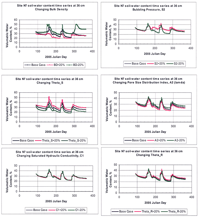
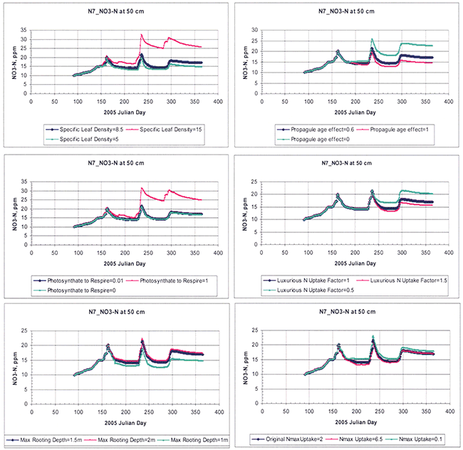
Figure 15--Sensitivity analysis of selected crop-growth parameters as exemplified for a random root-zone depth of 50 cm for site N7. Each variable was increased or decreased by a certain amount around an estimated base or initial value.
For hydraulic parameters, bulk density, saturation water content (θs), and the Brooks and Corey parameters λ and ψa were the most sensitive, whereas saturated hydraulic conductivity (Ksat) and residual water content (θr) were the least sensitive.
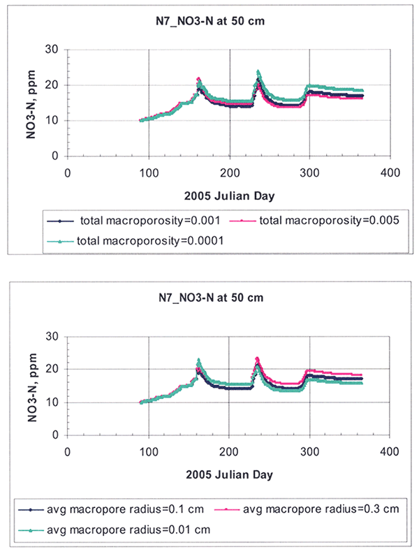
For the macropore parameters, the total macroporosity fraction and the average size of pore radii were the most sensitive (Fig. 16). Macroporosity had minimal effect on soil water content, but had appreciable effect on nitrogen distribution. Macropore flow is generated only during heavy rainfall events in the model. The major hydrologic effect of introducing macropores in the model is to reduce surface runoff.
Figure 16--Macropore sensitivity analysis as exemplified for a random root-zone depth of 50 cm for site N7.
Ahuja and Williams (1991) and Williams and Ahuja (2003) found that the soil water retention curves as described by the Brooks and Corey equations could be simply described by the pore size distribution index, λ. The importance of λ was used for scaling water infiltration and redistribution (Kozak and Ahuja, 2005) and for scaling evaporation and transpiration across soil textures (Kozak et al., 2005). Because of the relatively high sensitivity of parameters θs and λ, both of which are fitted (as opposed to experimentally measured) parameters, we decided to use primarily the λ-parameter and secondarily the θs parameter to calibrate our model.
For the plant-growth parameters, the specific leaf density, CLA (i.e., the amount of biomass needed to obtain a leaf area index, LAI = 1), the proportion of daily respiration as a function of photosynthesis, Φ (that maintains N uptake while decreasing biomass accumulation), the propagule age effect, Ap (that may result in increased photosynthesis efficiency during propagule development and thus increased yield, while above-ground biomass is kept constant), the luxurious nitrogen uptake factor (that starts 100 days after corn planting and allows the crop to take up exactly as much N or more or less than it needs), and the maximum depth of roots were the most sensitive. The seed-age effect (same as propagule-age effect but affects photosynthesis later in growing season), minimum leaf stomatal resistance (that is resistance to movement of water through leaf stomata), and the nitrogen sufficiency index (i.e., the fraction of the difference between the ideal and minimum N content of the crop) were the least sensitive.
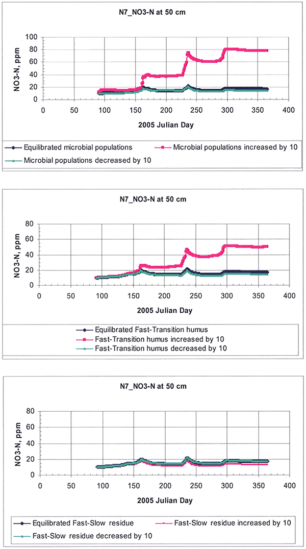
For the organic matter/nitrogen-cycling parameters, the aerobic heterotroph microbial population (that is, organisms capable of deriving carbon and energy from organic compounds, and growing only in the presence of molecular oxygen) and the transition and fast humus were the most sensitive parameters, as shown in Figure 17.
Figure 17--Sensitivity analysis of organic matter pools as exemplified for a random root-zone depth of 50 cm for site N7. The size of each pool was increased or decreased by one order of magnitude around the equilibrium base value.
Of course, the irrigation and fertilization rates were very sensitive inputs.
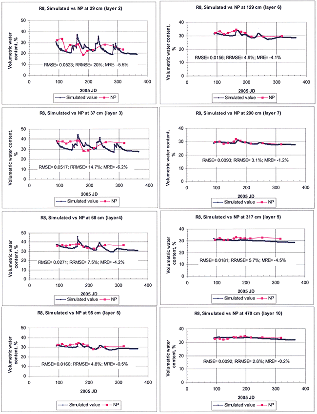
The simulated and observed moistures for the various individual layers are shown in Figures 18 and 19, for sites N7 and R8, respectively. Although for the upper layers of the soil in both sites the RRMSE and other error measures were relatively high, they much improved at increasing depths, as shown in the figures for the deeper layers. In addition, the simulation results, especially for site R8, show a slight negative bias or underprediction, as indicated by the negative value of the MRE statistic. In order to economize space from here onwards, we present simulation results from site N7 in more detail (for which we have relatively more detailed hydraulic-property data, resulting in generally and relatively somewhat better simulation results than for site R8).
Figure 18--Comparison of model-simulated and field-measured soil water contents at various soil depths for site N7. Three statistical indices, root mean square error (RMSE), relative RMSE (RRMSE), and mean relative error (MRE), all defined in the text, are used to quantify the goodness of fit of model parameterization.
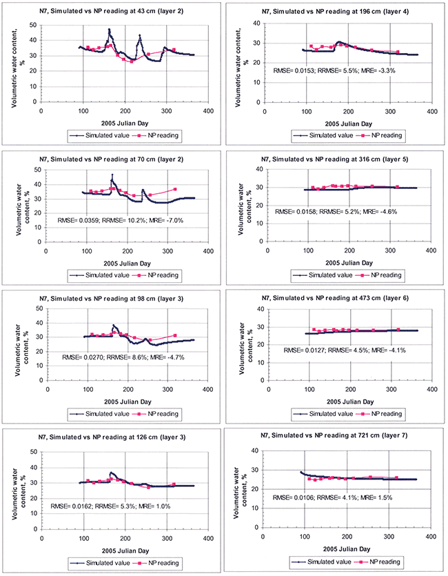
Figure 19--Comparison of model-simulated and field-measured soil water contents at various soil depths for site R8. Three statistical indices, root mean square error (RMSE), relative RMSE (RRMSE), and mean relative error (MRE), all defined in the text, are used to quantify the goodness of fit of model parameterization.
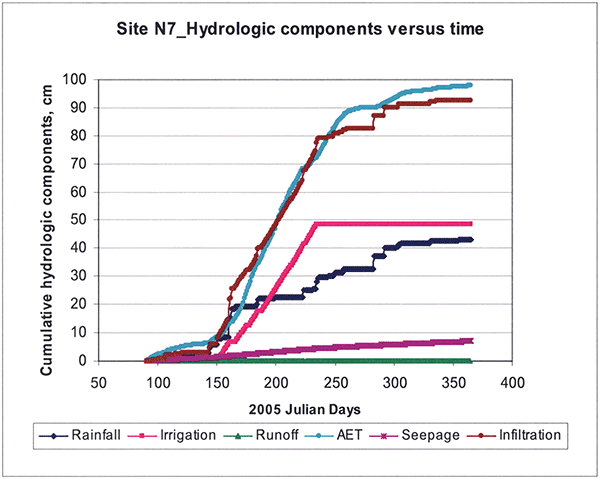
The simulated cumulative water budget components for the 2005 growing season are shown in Figure 20, where you notice that the runoff component is negligible during 2005.
Figure 20--Simulated cumulative hydrologic components for site N7 during the 2005 growing season.
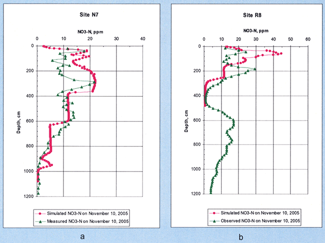
The simulated and measured soil nitrate profiles in the fall of 2005 in sites N7 and R8, both of which were planted in corn in April and harvested at the end of September are shown in Figure 21. For the case of site N7, the model approximated the main patterns of the nitrate depth profile fairly well, but not the observed detailed patterns. The results for site R8 were not as good as those for site N7, although they may be considered acceptable. As mentioned previously, we did not have hydraulic property data for the deeper R8 soil profile (only down to ~4.8 m), and as explained in the section on waterretention parameters in Sophocleous et al. (2006), some outside lab-determined hydraulic property data for that site were questionable.
Figure 21--Measured and simulated soil nitrate-nitrogen profiles at (a) site N7 (simulated depth 1080 cm) and (b) site R8 (simulated depth 484 cm) during the soil-sampling date of November 10,2005, following com harvest.
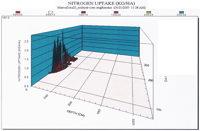
The simulated temporal distribution of nitrogen losses are shown in Figure 22, whereas the simulated spatial and temporal nitrogen uptake are shown in Figure 23.
Figure 22--Simulated temporal distribution of nitrogen losses (volatilization, denitrification, deep seepage) at site N7 during the 2005 corn-growing season.
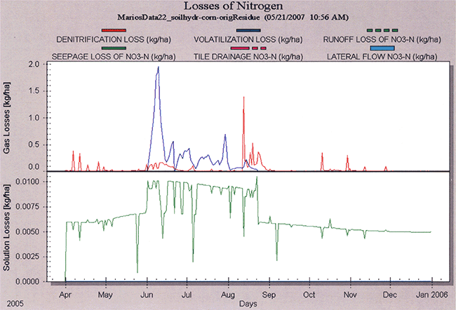
Figure 23--Three-dimensional diagram indicating the simulated spatial and temporal distribution of nitrogen uptake.
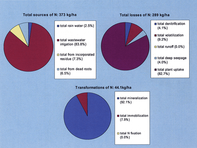
The model-estimated soil nitrogen balance is shown in Figure 24. The major source of nitrogen is the applied wastewater effluent that added more than 312 kg/ha during 2005 at site N7. The major nitrogen losses are from plant uptake, and secondarily from volatilization and deep seepage. Mineralization (that is, conversion of organic nitrogen that is present in soil organic matter, crop residues, and applied effluent to inorganic nitrogen, such as ammonium nitrogen, as a result of microbial decomposition) is the major transformation of nitrogen. However, large amounts of nitrate exist in the unsaturated soil profile as can be seen from Figure 7. The model-estimated storage of nitrate-nitrogen in the 10.8-m-deep soil profile analyzed in this model was more than 1500 kg/ha.
Figure 24--Simulated soil nitrogen balance components for site N7 during the 2005 growing season.
Once an agricultural system is adequately calibrated and tested, it has the potential for use in evaluation of alternative crop-soil management practices for the location of interest in terms of their production potential and impact on the environment (Hu et al., 2006). Because of the limited data we had available for calibrating and checking the RZWQM model, the results presented here should be considered preliminary.
Historical and current sampling of nitrogen in the soil at the wastewater-irrigated sites shows increased accumulation of inorganic nitrogen in the soil profile with time (see also Fig. 7), which indicates that the inorganic nitrogen left in the soil at harvest is not taken up completely by the subsequent crop. This residual nitrogen is subject to leaching to ground water when rainfall, especially of high intensity that enhances macropore flow, occurs between crop seasons. Numerical simulations indicated consistent increases in nitrogen losses due to volatilization (primarily) and deep seepage and denitrification (secondarily) with increased nitrogen application rates (see also Figs. 22-24).
Nitrogen Use Efficiency (NUE) is a term used to indicate the relative balance between the amount of fertilizer N taken up and used by the crop versus the amount of fertilizer N "lost." Nitrogen Use Efficiency in this report is defined as follows (Hu et al., 2006):
NUE = [(Plant N uptake under a particular N treatment) - (plant N uptake under no N fertilization)] / (amount of N applied) (8)
The RZWQM model was run with a zero-N treatment, and the results were used in the NUE computations.
Differences in predicted grain yields, plant N uptake, residual soil profile N, volatilization, and other N losses with different irrigation and fertilization treatments were analyzed using the RZWQM model and are summarized in Table 3. There is some uncertainty as to the total amount of fertilization applied in the fields. According to OMI lab analyses (see also Fig. 8 and Appendix A), the total N applied during the 2005 irrigation season was 434.5 kg/ha, According to Servi-Tech lab analyses (Appendix A, F. Vocasek, March 2007 written communication), the total was 312.4 kg/ha, To somewhat resolve this discrepancy, we adopted the Servi-Tech total but employed the OMI lab proportions of NO3, NH3, and organic nitrogen constituents of treated wastewater applied for irrigation (fertigation). The N balance components and NUE for both of the totals mentioned above are shown in Table 3. In addition, several management scenarios were simulated using reduced fertilization treatments of 50% of those OMI- and Servi-Tech-based wastewater-N totals mentioned above, as well as 75% and 50% reduced irrigation totals while maintaining the same irrigation scheduling.
Table 3--Nitrogen inputs and losses predicted by RZWQM for the 2005 crop season for site N7 for current irrigation, 75% irrigation, and 50% irrigation, and various levels of nitrogen fertilization through the irrigation LEPA system.
| Description of method | Total N Input (kg/ha) | Total N losses (kg/ha) | NUEc% | |||||||||||||
|---|---|---|---|---|---|---|---|---|---|---|---|---|---|---|---|---|
| Crop yield (kg/ha) |
Percent change in crop yield |
Storage (10.8m- profile) |
Rain | Fertigationb | Mineralization | Percent change in mineralization |
Plant uptake |
Percent change in plant uptake |
Deep seepage |
Percent change in deep seepage |
Denitrification | Percent change in denitrification |
Volatilization | Percent change in volatilization |
||
| 1. Full rate irrigationa, full rate fertilizationb |
6030.3 | --- | 1518.5 | 9.4 | 312.4 | 40.6 | --- | 239.0 | --- | 11.6 | - | 11.9 | --- | 26.5 | --- | 17.12 |
| 2. Full rate irrigation, 50% fertilization | 5961.8 | -1.14 | 1465.8 | 9.4 | 156.9 | 40.9 | 0.73 | 251.8 | 5.32 | 11.6 | 0.0 | 7.8 | -34.59 | 5.1 | -80.66 | 42.19 |
| 3. Full rate irrigation, zero fertilization | 5198.8 | -13.79 | 1426.3 | 9.4 | --- | 40.9 | 0.71 | 185.6 | -22.37 | 11.6 | -0.00 | 5.4 | -54.15 | 0.01 | -99.95 | - |
| 4. 75% irrigation, full rate fertilization | 6067.9 | --- | 1519.7 | 9.3 | 312.4 | 42.8 | --- | 236.6 | --- | 11.6 | --- | 10.5 | --- | 30.7 | --- | 17.47 |
| 5. 75% irrigation, 50% fertilization | 6006.7 | -1.01 | 1469.6 | 9.3 | 156.9 | 43.1 | 0.56 | 257.5 | 8.82 | 11.6 | 0.00 | 7.3 | -30.55 | 5.9 | -80.72 | 48.08 |
| 6. 75% irrigation, zero fertilization | 5367.5 | -11.54 | 1427.8 | 9.3 | --- | 43.4 | 1.37 | 182.0 | -23.06 | 11.6 | 0.01 | 5.3 | -49.63 | 0.01 | -99.96 | --- |
| 7. 50% irrigation, full rate fertilization | 6002.8 | -0.46 | 1519.7 | 9.3 | 312.4 | 44.5 | 9.44 | 222.7 | -6.85 | 11.5 | -0.71 | 9.9 | -16.77 | 38.6 | 45.38 | 13.75 |
| 8. 50% irrigation, 50% fertilization | 5969.8 | -1.00 | 1472.0 | 9.3 | 156.9 | 44.7 | 9.95 | 255.3 | 6.81 | 11.5 | -0.71 | 7.0 | -41.08 | 7.4 | -72.28 | 48.18 |
| 9. 50% irrigation, zero fertilization | 5507.7 | -8.67 | 1428.5 | 9.3 | --- | 45.2 | 11.16 | 179.7 | -24.82 | 11.5 | -0.71 | 5.2 | -56.11 | 0.01 | -99.95 | --- |
|
a Full rate of 2005-season irrigation = 48.55 cm b Full rate of 2005-season fertigation = 312.4 kg/ha c Nitrogen Use Efficiency |
||||||||||||||||
| Description of method | Total N Input (kg/ha) | Total N losses (kg/ha) | NUEf% | |||||||||||||
|---|---|---|---|---|---|---|---|---|---|---|---|---|---|---|---|---|
| Crop yield (kg/ha) |
Percent change in crop yield |
Storage (10.8m- profile) |
Rain | Fertigatione | Mineralization | Percent change in mineralization |
Plant uptake |
Percent change in plant uptake |
Deep seepage |
Percent change in deep seepage |
Denitrification | Percent change in denitrification |
Volatilization | Percent change in volatilization |
||
| 10. Full rate irrigationd, full rate fertilizatione |
6054.4 | --- | 1559.6 | 9.4 | 434.5 | 40.6 | --- | 231.3 | --- | 11.6 | --- | 15.0 | --- | 58.7 | --- | 10.52 |
| 11. Full rate irrigation, 50% fertilization | 6017.8 | -0.60 | 1486.1 | 9.4 | 217.3 | 40.8 | 0.42 | 254.9 | 10.20 | 11.6 | 0.0 | 9.1 | -39.12 | 11.3 | -80.83 | 31.91 |
| 12. Full rate irrigation, zero fertilization | 5198.8 | -14.1 | 1426.3 | 9.4 | --- | 40.9 | 0.80 | 185.6 | -19.77 | 11.6 | -0.00 | 5.4 | -63.76 | 0.01 | -99.98 | --- |
| 13. 50% irrigation, full rate fertilization | 5995.0 | -0.98 | 1553.1 | 9.3 | 434.5 | 44.4 | 9.37 | 237.8 | 2.80 | 11.5 | -0.71 | 12.1 | -19.67 | 84.4 | 43.75 | 13.36 |
| 14.50% irrigation, 50% fertilization | 5978.8 | -1.25 | 1489.6 | 9.3 | 217.3 | 44.5 | 9.74 | 240.5 | 3.96 | 11.5 | -0.71 | 8.0 | -46.58 | 16.2 | -72.39 | 27.96 |
| 15.50% irrigation, zero fertilization | 5507.7 | -9.03 | 1428.5 | 9.3 | --- | 45.2 | 11.25 | 179.7 | -22.30 | 11.5 | -0.71 | 5.2 | -65.31 | 0.01 | -99.98 | --- |
|
d Full rate of 2005-season irrigation = 48.55 cm e Full rate of 2005-season fertigation = 434.5 kg/ha f Nitrogen Use Efficiency |
||||||||||||||||
We see that reducing fertilization by 50% using the same 2005 irrigation scheduling increases NUE while keeping relative crop yield nearly constant with a decrease of only 1 % of maximum simulated yield (see Table 3, items 2, 5, 8, 11, and 14). Lowering fertigation from 435 kg/ha (Table 3, item 10) to 312 kg/ha (Table 3, item 1), to 217 kg/ha (Table 3, item 11), to 157 kg/ha (Table 3, item 2) consistently increased NUE (10.5%, 17.1 %, 31.9%, 42.2%, respectively). Reducing irrigation total amount while keeping fertilization levels at 157 kg/ha further increases NUE from 42.2% (at full irrigation amount--Table 3, item 2) to 48.1% (at 75% of full irrigation amount-Table 3, item 5) to only 48.2% (at 50% of full irrigation amount--Table 3, item 8). This last result indicates that such a drastic irrigation reduction (50%) may not be necessary, as nearly the same NUE is obtained with 75% irrigation reduction.
It seems that reducing the fertilization levels at the study sites to around 150 kg/ha increases the NUE significantly. Such lower fertilization rates can be achieved by blending treated wastewater effluent with freshwater from the underlying High Plains aquifer. In addition, decreasing the amount of irrigation water applied by approximately 25%, while using reduced fertilization rates, further increases NUE.
Sophocleous, M. A., Townsend, M. A., Willson, T., and Vocasek, F., and Zupancic, J., 2006, Fate of nitrate beneath fields irrigated with treated wastewater in Ford County, Kansas: First-year Progress Report to KWRI, 62 p.
Sophocleous, M. A., Townsend, M. A., Willson, T., and Vocasek, F., 2006, Fate of nitrate beneath fields irrigated with treated wastewater in Ford County, Kansas: 23rd Annual Water and the Future of Kansas Conference, Topeka, KS, March 16,2006.
Sophocleous, M. A., Townsend, M. A., Willson, T., and Vocasek, F., 2006, Preferential flow and transport of nitrate beneath fields irrigated with treated wastewater in Ford County: Geological Society of America, GSA Abstracts with Program, v. 38, no. 7, p. 40.
Townsend, M. A., Macko, S. A., Sophocleous, M. A., Vocasek, F., Schuette, D., and Ghijsen, R., 2006, Documenting seasonal variation at a wastewater irrigation site through stable isotopes: Geological Society of America, GSA Abstracts with Program, v. 38, no. 7, p. 40.
Sophocleous, M. A., Townsend, M. A., and Vocasek, F., 2007, Treated wastewater and nitrate transport beneath irrigated fields near Dodge City, Kansas: Water and the Future of Kansas Conference, March 15, 2007, Topeka, KS.
Townsend, M. A., Macko, S. A., Sophocleous, M. A., Vocasek, F., Schutte, D., and Ghijsen, R., 2007, Variations in water chemistry and plant uptake of nitrogen at a wastewater irrigation site: Water and the Future of Kansas Conference, March 15, 2007, Topeka, KS.
Note: A journal manuscript based on this report and additional ongoing work is under preparation.
See Publications and Presentations above. In addition, Dodge City TV broadcasting news services recorded our dye-tracer experiments in November 2005 and interviewed co-PI Fred Vocasek on this project. See also Student Support below.
A graduate student in the School of Engineering of the University of Kansas is being supported by this project. Main duties include data processing and numerical modeling. An MS non-thesis project based on this study is now being pursued by the graduate student (Ashok KC). An additional hourly student from Kansas State University based in the Garden City Agricultural Experiment Station has been supported for conducting periodic neutron moisture-content readings at the field sites.
Numerous people and agencies assisted us during the conduct of this study, and they are listed below as a token of our gratitude.
Abrahamson, D. A., Radcliffe, D. E., Steiner, J. L., Cabrera, M. L., Hanson, J. D., Rojas, K. W., Schomberg, H. H., Fisher, D. S., Schwartz, L., and Hoogenboom, G., 2005, Calibration of the Root Zone Water Quality Model for simulating tile drainage and leached nitrate in the Georgia Piedmont: Agron. J., v. 97, p. 1584-1602.
Ahuja, L. R., DeCoursey, D. G., Bames, B. B., and Rojas, K. W., 1993, Characteristics of macropore transport studied with the ARS Root Zone Water Quality Model: Transactions of the ASAE, v. 36, no. 2, p. 369-380.
Ahuja, L. R., and Ma, L., 2002, Parameterization of agricultural system modelsCurrent approaches and future needs; in, Agricultural System Models in Field Research and Technology Transfer, L. R. Ahuja, L. Ma, and T. A. Howell, eds.: Lewis Publishers, p. 273-316.
Ahuja, L. R., Rojas, K. W., Hanson, J. D., Shaffer, M. J., and Ma, L., eds., 2000, Root Zone Water Quality Model-Modeling management effects on water quality and crop production: Water Resources Publications, LLC, Highlands Ranch, CO, 372 p.
Ahuja, L. R., and Williams, R. D., 1991, Scaling of water characteristic and hydraulic conductivity based on Gregson-Hector-McGowan approach: Soil Sci. Soc. Am. J., v. 55, p. 308-319.
Brooks, R. H., and Corey, A. T., 1964, Hydraulic properties of porous media: Hydrol. Paper 3, Colorado State University, Fort Collins, CO.
Dodge, D. A., Tomasu, B. I., Haberman, R. L., Roth, W. E., and Baumann, J. B., 1965, Soil survey Ford County, Kansas: U.S. Department of Agriculture, Soil Conservation Service, Series 1958, no. 32, 84 p.
Farahani, H. J. and Ahuja, L. R., 1996, Evapotranspiration modeling of partial canopy/residue covered field: Transactions of the ASAE, v. 39, p. 2051-2064.
Flury M., Fluhler, H., Jury, W. A., and Leuenberger, J., 1994a, Susceptibility of soils to preferential flow of water--A field study: Water Resources Research, v. 30, no. 7, p. 1945-1954.
Flury, M., and Fluhler, H., 1994, Brilliant blue FCF as a dye tracer for solute transport studies--A toxicological overview: Environ. Qual., v. 23, p. 1108-1112.
Flury, M., and Fluhler, H., 1995, Tracer characteristics of brilliant blue FCF: Soil Sci. Soc. Am. J., v. 59, p. 22-27.
Flury, M., and Wai, N. N., 2003, Dyes as tracers for vadose zone hydrology: Reviews of Geophysics, v. 41, p. 1/1002.
Hanson, J. D., 2000, Generic crop production; in, Root Zone Water Quality Model, L. R. Ahuja et al., eds.: Water Resources Publications, Highland Ranch, CO, p. 81-118.
Hanson, J. D., Rojas, K. W., and Shaffer, M. J., 1999, Calibrating the Root Zone Water Quality Model: Agron. J., v. 91, p. 171-177.
Hu, C., Saseendran, S. A., Green, T. R., Ma, L., Li, X., and Ahuja, L. R., 2006, Evaluating nitrogen and water management in a double-cropping system using RZWQM: Vadose Zone Journal, v. 5, p. 493-505.
Kozak, J. A., and Ahuja, L. R., 2005, Scaling of infiltration and redistribution across soil textural classes: Soil Sci. Soc. Am. J., v. 69, p. 816-827.
Kozak, J., Ahuja, L. R., Ma. L., Green, T. R., 2005, Scaling and estimation of evaporation and transpiration of water across soil texture classes: Vadose Zone J., v. 4, p. 418-427.
Ma, L., Shaffer, J. J., Boyd, J. K., Waskom, R., Ahuja, L. R., Rojas, K. W., and Xu, C., 1998, Manure management in an irrigated silage corn field-Experiment and modeling: Soil Sci. Soc. Am. J., v. 62, p. 1006-1017.
Ma, L., Ascough, J. C., II, Ahuja, L. R., Shaffer, M. J., Hanson, J. D., and Rojas, K. W., 2000, Root Zone Water Quality Model sensitivity analysis using Monte Carlo Simulation: Transactions of the ASAE, v. 43, no. 4, p. 883-895.
Malone, R. W., Ma, L., Heilman, P., Karlen, D. L., Kanwar, R. S., Hatfield, J. L., in press, Simulated N management effects on corn yield and tile-drainage nitrate loss: Geoderma, in press.
Mueller, D. K. and Helsel, D. R., 1996, Nutrients in the nation's waters--Too much of a good thing?: U.S. Geological Survey, Circular 1136, 24 p. [available online]
Petersen, C. T., Hansen, S., and Jensen, H. E., 1997, Depth distribution of preferential flow patterns in a sandy loam soil as affected by tillage: Hydrology and Earth System Sciences, v. 4, p. 769-776.
Schaap, M. G., Leij, F. J., and van Genuchten, M. Th., 2001, ROSETTA--A computer program for estimating soil hydraulic parameters with hierarchical pedotransfer functions: Jour. Hydrology, v. 251, p. 163-176.
Schwartz, R. C., Mcinnes, J. J., Juo, A. S. R., and Cervantes, C. E., 1999, The vertical distribution of a dye tracer in a layered soil: Soil Science, v. 164, no. 8.
Shipitalo, M. J. and Ewards, W. M., 1996, Effects of initial water content on macropore/matrix flow and transport of surface-applied chemicals: J. Environ. Qual., v. 25, p. 662-670.
Sophocleous, M. A., Townsend, M. A., Willson, T., Vocasek, F., and Zupancic, J., 2006, Fate of nitrate beneath fields irrigated with treated wastewater in Ford County, Kansas: First-year Progress Report to KWRI; Kansas Geological Survey, Open-file Report 2007-14,62 p.
U. S. Geological Survey, 2004, NAWQA, Significant findings irrigated agriculture land-use study--central High Plains: U.S. Geological Survey, http://co.water.usgs.gov/nawqa/hpgw/html/SIGFINDS.html
van Genuchten, M. Th., 1980, A closed-form equation for predicting the hydraulic conductivity of unsaturated soils: Soil Sci. Am. J., v. 44, p. 892-898.
van Genuchten, M. Th., Leij, F. J., and Yates, S. R., 1991, The RETC code for quantifying the hydraulic functions of unsaturated soils: U.S. Environmental Protection Agency, Report 600/2-91/065.
Walker, S. E., Mitchell, J. K., Hirschi, M. C., and Johnsen, K. E., 2000, Sensitivity analysis of the Root Zone Water Quality Model: Transactions of the ASAE, v. 43, no. 4, p. 841-846.
Williams, R. D., and Ahuja, L. R., 2003, Scaling and estimating the soil water characteristic using a one-parameter model; in, Scaling Methods in Soil Physics, Y. Pachepsky, D. E. Radcliffe, and H. M. Se1im, eds.: CRC Press, Boca Raton, FL, p. 35-48.
Zupancic, J. W., and Vocasek, F. F., 2002, Dealing with changes in volume and quality of effluent at the Dodge City wastewater recycling project over the last sixteen years-1986 through 2001: 2002 Technical Conference Proceedings of the Irrigation Association, New Orleans, Louisiana.
Effluent composition (nutrient variables) applied at the study sites N7 and R8 during 2005 and 2006.
Table A1--Effluent composition, irrigation stations, nutrient variables (OMI Lab).
| Sample location |
Sample date |
TKN mg/L |
NH3-N mg/L |
NO3-N mg/L |
Organic-Nitrogen mg/L |
PO4-P mg/L |
|---|---|---|---|---|---|---|
| Irrigation station# 1 (irrigating site N7) |
4/14/2005 | 88.0 | 85.0 | 0.7 | 3.0 | 11.4 |
| 5/17/2005 | 79.0 | 57.9 | 7.3 | 10.8 | ||
| 6/21/2005 | 81.0 | 64.0 | 27.0 | 17.0 | 9.6 | |
| 7/22/2005 | 81.0 | 76.9 | 0.0 | 4.1 | 10.7 | |
| 8/30/2005 | 80.0 | 65.3 | 1.7 | 14.7 | 9.8 | |
| 9/23/2005 | 20.0 | 4.5 | 23.4 | 15.5 | 8.9 | |
| 10/28/2005 | 65.0 | 55.2 | 9.8 | 10.4 | ||
| 8/3/2005 | 80.0 | 70.0 | <1.0 | 10.0 | ||
| 4/27/2006 | 91.0 | 85.7 | 0.0 | 5.3 | 11.2 | |
| 5/26/2006 | 90.0 | 80.9 | 0.0 | 9.1 | 10.8 | |
| 6/15/2006 | 130.0 | 86.3 | 0.0 | 43.7 | 11.7 | |
| 7/21/2006 | 95.0 | 90.2 | 0.0 | 4.8 | 12.5 | |
| 8/11/2006 | 100.0 | 80.2 | 0.0 | 19.8 | 13.9 | |
| 9/21/2006 | 110.0 | 85.8 | 0.0 | 24.2 | 17.0 | |
| 10/25/2006 | 110.0 | 90.0 | 0.0 | 20.0 | 16.7 | |
| Irrigation station #2 (irrigating site R8) |
6/21/2005 | 30.0 | 18.8 | 13.8 | 11.2 | 10.0 |
| 7/22/2005 | 29.0 | 26.2 | 22.8 | 2.8 | 10.9 | |
| 8/30/2005 | 57.0 | 33.3 | 0.8 | 23.8 | 8.6 | |
| 9/23/2005 | 20.0 | 0.3 | 24.8 | 19.7 | 6.2 | |
| 10/28/2005 | 15.0 | 0.4 | 14.6 | 4.8 | ||
| 8/3/2005 | 50.0 | 20.0 | 20.0 | 10.0 | 26.0 | |
| 4/27/2006 | 40.0 | 32.5 | 3.6 | 7.5 | 8.7 | |
| 5/26/2006 | 20.0 | 12.4 | 25.6 | 7.7 | 9.2 | |
| 6/15/2006 | 51.0 | 36.9 | 0.0 | 14.1 | 10.9 | |
| 7/21/2006 | 79.0 | 68.2 | 1.0 | 10.8 | 11.3 | |
| 8/11/2006 | 65.0 | 54.2 | 0.0 | 10.8 | 12.0 | |
| 9/21/2006 | 72.0 | 42.5 | 1.3 | 29.5 | 11.3 |
Kansas Geological Survey, Geohydrology
Placed online July 14, 2014
Comments to webadmin@kgs.ku.edu
The URL for this page is http://www.kgs.ku.edu/Hydro/Publications/2007/OFR07_25/index.html