Kansas Geological Survey, Open-file Report 2007-14
Next Page--Appendices...
1 Kansas Geological Survey
2 Kansas State University
3 Servi-Tech Agri/Environmental Consulting Services
4 Agronomy Solutions LCC
First-Year Progress Report to KWRI (March 1 , 2005 - February 28, 2006)
Kansas Geological Survey, Open-File Report 2007-14
This report is available as an Acrobat PDF file (16 MB).
May 2006
With increasingly limited groundwater resources, reuse of treated wastewater provides an alternative source of water for irrigation of crops and landscaping. A long-term irrigation project with treated wastewater south of Dodge City in Ford County, Kansas, is the focus of this study. The use of treated wastewater in that area has resulted in high nitrate concentrations (10-50 mg/kg) throughout the upper 50-ft profile but at varying concentrations, suggesting that preferential flow processes have occurred at the proposed study area. Evaluation of the environmental impact of such land-use strategies needs to be made in order to determine if and when this process may impact usable groundwater at depth. The goal of this project is to estimate the leaching rates and time of arrival of N- (and Cl-) contaminants using preferential flow and N-cycling numerical modeling in combination with field and laboratory measurements at the study sites. This approach also will help to identify key parameters and processes that influence N losses in agricultural soils and can facilitate evaluation of the environmental impact of different land use practices.
To achieve this goal we collected deep cores for physical and chemical properties characterization, including using the Geoprobe capabilities for electrical conductivity profiling; performed dye tracer experiments; installed neutron moisture probe access tubes and regularly collected soil moisture data; and obtained soil chemical data, crop and irrigation application rate information, climatic data, and other additional information from the ongoing study in the area, which is managed by the two consultant co-PIs on this project. This report details the data collection and analysis during the 1st year of this project. All these data are now being used in the comprehensive N-cycling model RZWQM (which also accounts for preferential flow and transport) to identify key parameters and processes that influence N losses in the study area. This second phase of this project is ongoing and will be reported in a later update of this report.
Results from this study will assist in determining leaching rates and fate of nitrogen in the High Plains aquifer from wastewater irrigation, provide additional data for enhancing the nitrogen budget for the area in question, and assist in providing information for other areas where there is an interest in using reclaimed water for landscape irrigation as a means to conserve water or for disposal purposes.
Table of contentsAbstract
1. Introduction
2. Objectives
3. Statement of the problem
4. Related Research
5. Methodology
5A. Field monitoring sites
5B. Soil sampling and analyses
5C. Neutron probe calibration
5D. Water Sampling and Chemical Analysis Methods
5E. Dye-tracer experiments
5F. Numerical simulation
5F.1 RETC and ROSETTA retention-curve estimation
5G. Statistical methods
6. Results: Significant findings
6A. Soil Physical-Chemical properties
6B. Soil Hydraulic properties
6B.1 Saturated hydraulic conductivity
6B.2 Retention curve data
6B.3 Water retention parameters
6C. Soil moisture profiles
6D. Dye-tracer experiment results
6E. Soil nitrate, chloride, and electrical conductivity profiles
6F. Water quality
6G. Land use/farming practices
Publications and Presentations
Information Transfer
Student Support
Acknowledgments
References
Appendix A. Soil Profile Descriptions
Appendix B. Water chemistry for monitoring, domestic, and irrigation wells near study areas, Dodge City, Kansas, Spring 2005
Appendix C. Water chemistry analyses for Reservoirs and Irrigation well discharge points at OMI wastewater treatment plant, Dodge City, Kansas 2004-2005.
Appendix D. Lysimeter water chemistry for sites N7 and R8, Summer 2005
With increasingly limited groundwater resources, reuse of treated wastewater provides an alternative source of water for irrigation of crops and landscaping. In addition, utilization of the nutrients in recycled wastewater as fertilizer results in less application of fertilizer to a plant system.
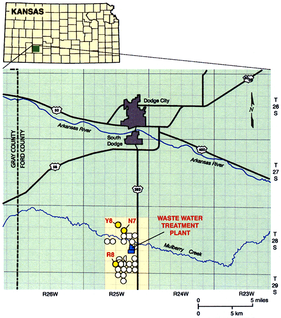
A long-term irrigation project using treated municipal wastewater has been ongoing south of Dodge City in Ford County since the mid-1980s and is shown in Fig. 1. This area is underlain by the High Plains aquifer, and constitutes the study area for this project. Use of the treated wastewater, which includes inputs from both the municipality of Dodge City and a meat-packing plant, has resulted in relatively high soil nitrate-nitrogen concentrations (10-50 mg/kg) in the soil profile at the sites irrigated with this treated wastewater effluent (Zupancic and Vocasek, 2002). Evaluation of the environmental impact of such land-use strategies needs to be made in order to determine if and when this process may impact usable groundwater at depth and what management changes may need to be made to slow down the downwards N migration.
Figure 1--Location of the study area.
The study area overlies the High Plains aquifer with depth to water in the range of 75 to 150 ft. The overlying soils are predominantly Harney and Ulysses silt loams (Dodge et al., 1965). Although this area has a deep water table and soils with a silty clay component, there is evidence that nitrate is migrating through the vadose zone. USGS National Water-Quality Assessment studies in the Central High Plains aquifer region indicate that nitrate from fertilizer sources and animal waste has reached the Ogallala portion of the High Plains aquifer most likely due to increased recharge from irrigation but also because of preferential flow processes (USGS, 2004). Work by the Kansas Geological Survey indicates that: (1) nitrate has reached the Ogallala aquifer in northwest Kansas (Townsend et al., 1996); (2) nitrate is migrating through the shallow vadose zone to the High Plains aquifer in south-central Kansas (Sophocleous et al., 1990a, 1990b) and (3) an overview of nitrate in Kansas groundwater (Townsend and Young, 2000) shows levels above the 2 mg/L background level (Mueller and Helsel, 1996) in several major aquifers in the state, including the High Plains.
Because of the importance of the High Plains aquifer as a source of drinking and irrigation water, the quality of the water is an important issue. Determining the rate of movement of contaminants to the groundwater is a difficult task. Field investigations in combination with modeling constitute a promising methodology for estimation of leaching rates and time of arrival of contaminants. Modeling can also better identify key parameters and processes that influence N losses in agricultural soils and can facilitate evaluation of the environmental impact of different land-use practices.
Therefore, the objectives of this project are:
The Dodge City Wastewater Treatment Plant (DCWTP) is collecting wastewater from the City and a meat packing plant into a collection station. The collected wastewater is piped about 11 miles south of the city into a wastewater treatment facility (Fig. 1). This facility consists of three covered anaerobic digesters (i.e., covered lagoons with impermeable covers that trap gas produced during decomposition of the liquid effluent) and three aeration basins. The treated water is stored in storage lagoons with a capacity of more than 2800 acre-ft. A pumping system, consisting of several electric, centrifugal pumps distributes the water to irrigate more than 2700 acres of cropland in 25 fields (Fig. 1). The system is managed by Operations Management International (OMI) and the agronomic firm Servi-Tech, Inc. under contracts with the City.
Early results of soil monitoring by Servi-Tech company personnel showed that significant amounts of nitrate-N were passing beyond the upper 5-feet of the soil profile (Zupancic and Vocasek, 2002). Deeper coring was then undertaken, and soil nitrate-N concentrations exceeding 10 mg/kg have been detected down to depths of approximately 40 ft. Also, concentrations above the drinking water limit of 10 mg/L NO3-N have been found in groundwater from monitoring wells in the area (Zupancic and Vocasek, 2002).
Servi-Tech personnel have also noted macropores with diameters ranging from pinpoint size to nearly 0.25 inch in the undisturbed cores collected during sampling. These macropores are most numerous in the upper soil profile, but also occur at depths down to 40 or so ft. The interior of these macropores take on a brownish color after sampling, possibly from organic carbon anoxidation, suggesting these may be historic root channels.
Thus, the occurrences of nitrate at depth and the presence of macropores suggest the possibility that preferential flow processes through macropores bypassing the attenuating effect of the soil matrix are occurring.
Irrigation of secondarily treated wastewater is an acceptable, well-studied method of wastewater reuse. Land application of wastewater has been extensively studied both in the U.S.A. and abroad (Ayers and Westcott, 1989; Townsend, 1982; Hogg et al., 2003). Soil-profile monitoring at the Dodge City site began in 1987 during the second year of wastewater application. Soil-salinity impacts were the major concern in 1987, but nutrients (including nitrate) also were included in the monitoring program (Zupancic and Vocasek, 2002). The DCWTP capacity was quickly pushed beyond the design specifications and wastewater nitrogen concentrations increased about three-fold. Project-wide nitrogen budgets showed net nitrogen inputs exceeding crop nitrogen removals by 60% to 80% (Zupancic and Vocasek, 2002).
As mentioned before, the occurrences of nitrate at depth and the presence of macropores suggest the possibility that preferential flow processes have occurred. Various types of dyes have been used to stain the flow paths of water in soils to circumvent measurement difficulties of preferential flow due to tremendous spatial and temporal variability (Bouma et al., 1977; Flury et al., 1994). The results obtained from staining experiments clearly illustrate the complicated pattern of water movement with a very high spatial resolution.
The importance of macropores in preferential flow cannot be overstated. Macropores allow rapid gravitational flow of the free water available at the soil surface or above an impeding soil horizon, thus bypassing the soil matrix. Short circuiting to groundwater through macropores is of serious concern at present because of the possibilities of rapid transport of a portion of fertilizers, pesticides and other chemicals applied on the soil surface (Ahuja et al., 1993).
This concern has been exacerbated by the growing practice of minimum or no tillage, which allows chemical solutes in irrigation water applied on the soil surface to accumulate and to enter macropores at the surface. Plant residues on the surface and no tillage also enhances worm activity and allow worm holes and other macropore channels to stay open at the surface (Ahuja et al., 1993).
Preferential flow can be described using a variety of dual-porosity, dual-permeability, multiporosity, and/or multi-permeability models (Simunek et al., 2003). The main disadvantage of such models is that, contrary to models for a single pore region, they require more input parameters to characterize both macropore and micropore systems. However, little guidance is available as to how to obtain these parameters, either by direct measurement, a priori estimation, or some calibration technique (Simunek et al., 2003).
Standard procedures have not yet been established for macropore input parameters. Logsdon (2002) evaluated several methods to independently measure macropore parameters using soils from the Des Moines lobe with textures ranging from sandy loam to silty clay. Rawls et al. (1996) developed empirical equations to calculate macropore size/count, areal porosity, and macropore conductivity based on three levels of available data. Jarvis et al. (1997) presented guidance on parameter estimation of macropore-system properties for input into preferential flow models based on easily measured soil physical properties. We plan to implement these suggested parameter-estimation procedures in our study and evaluate their predictive accuracy.
The effects of macropore flow on nitrogen loading are not well investigated, although several models now exist that take transport through macropores into account (Larsson and Jarvis, 1999). Under non-fertilized conditions, we should expect leaching loads to be reduced because nitrogen is inherent to the soil, so that rainwater that rapidly bypasses the soil matrix will have a smaller NO3 concentration than the resident soil solution. With wastewater-nitrogen inputs though, the consequences of macropore flow are not very clear (Larsson and Jarvis, 1999).
Measurements of the soil hydraulic conductivity and/or soil-water retention curve are costly, time-consuming, and sometimes unreliable because of soil heterogeneity and experimental errors. Methods have been developed to estimate soil hydraulic properties from more easily measured soil properties (Wosten et al., 2001). These methods involve the use of pedotransfer functions (PTFs; see further in section 7 A.2.c). A number of PTFs can be found in the literature and can be classified according to the nature of the basic input soil properties and the method adopted to generate predictions (Wosten et al., 2001). A neural network approach to estimating PTFs is available in the ROSETTA software (Schaap et al., 2001) and was shown to be reasonably good for simulating soil-moisture variations in the field (Nemes et al., 2003), and therefore we plan to employ it in our study, as well as the popular RETC code (van Genuchten et al., 1991) for quantifying the hydraulic functions of unsaturated soils (see further in section 5F.1).
Land application of treated wastewater is a proven technology that is utilized world wide (Ayers and Westcot, 1989). Reuse of wastewater is particularly common in developing countries and in arid portions of the western United States (Bouwer, 1992). Generally water quality is improved by land application of wastewater and use of the soil as a filtering system for removal of microbes, organic and inorganic forms of nitrogen and other chemicals that can be detrimental to human health (Asano, 2006; Schreffler and Galeone, 2005, Avnimelech, 1993). In most situations nitrogen is utilized by plants and mineralized in soils. However, some studies such as the study in the Lake Tahoe region in California (Hayes and deWalle, 1993), excessive application of wastewater during the winter when the ground was frozen and plants were dormant resulted in an increase of conductivity, chloride, and nitrogen in groundwater in the area. In addition, in arid areas there always exists the possibility of enrichment of anions in the irrigation water due to evapoconcentration processes (Babcock et al., 2005, Bouwer, 1992; Hayes and DeWalle, 1993). The study area near Dodge City has been in operation since 1987. Salinity and leaching nitrate are continuously under observation and methods are changed as necessary to deal with the issues (Vocasek, 2006).
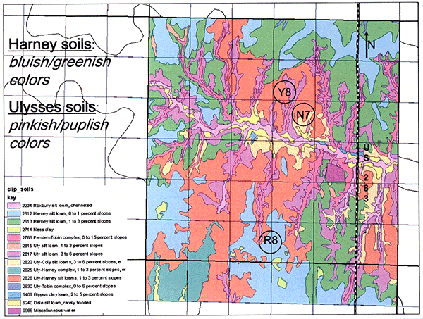
To analyze this nitrogen leaching problem further, we established two main monitoring sites, one in each of the two major loess-derived soil series in the project area, the Harney and the Ulysses soils (Fig. 2; the Harney silt loams are the bluish and greenish colors in the slide, whereas the Ulysses silt loams are the reddish and purplish colors). One of the sites, the R8 in Harney soils, has a long-term treated wastewater irrigation history (since 1986), whereas the other site, N7 in Ulysses soils, has a short-term treated wastewater irrigation history (since 1998). In addition, a third, control site, Y8, without any wastewater irrigation record, has also been established (Fig. 2).
During the first year of this project we concentrated on establishing and instrumenting the monitoring sites and collecting the basic data for our further analyses, and this is what this report will emphasize.
Figure 2--Map of soils in Ford County at study sites (Data downloaded from the NRCS Geospatial Data Gateway at http://datagateway.nrcs.usda.gov/).
We collected several deep cores, down to 50 ft, from each of the sites for a number of physical, chemical and future isotopic analyses (year 2). Analyses included: textural analysis, bulk density, percent total carbon, total Kjeldahl nitrogen, nitrate, ammonium, percent carbonate, cation exchange capacity, percent water content for various pressures, chloride, pH, electrical conductivity, sodium adsorption ratio, and others.
Soil analyses were done by the Natural Resources Conservation Services (NRCS) Lincoln Laboratory, by the Kansas State University Soil Testing Laboratory, and Servi-Tech laboratories. The NRCS Laboratory used the dry combustion method for Total Carbon (Ctot) determinations. The amount of carbonate in the soil is determined by treating the sample with HCl followed by manometrically measuring the evolved CO2. The amount of carbonate is then calculated as a CaCO3 equivalent basis. Values of total organic carbon (TOC) were determined by difference between total carbon and percent calcium carbonate (CaCO3) multiplied by 0.12, the fraction of carbon in calcium carbonate (i.e., TOC = Ctot - 0.12*CaCO3).
Cation exchange capacity (CEC) is a measure of the total quantity of negative charges per unit weight of the soil and is commonly expressed in units of milliequivalents per 100 g of soil (meq/100g) or centimoles per kilogram of soil (cmol(+)/kg). The Sodium Adsorption Ratio (SAR), i.e., the ratio of the molar concentration of the monovalent cation Na+ to the square root of the molar concentrations of the divalent Ca2+ and Mg2+ in the soil, divided by 2, is a measure of potential hazards from high sodium levels.
The soil bulk density down to 15.2 m (50 ft) was determined from collected cores of known diameter by cutting the core in 15.2-cm (6-in) increments, weighing them in the field, and then oven-drying them in the lab. KSU Southwest Agricultural Station and the NRCS Lincoln calculated bulk density using different methods. The values calculated by the KSU Southwest Agricultural Station were used for calibration of the neutron probe.
The deep cores (of 15.2-m total length), that were collected in April, 2005, were analysed by Servi-Tech for nitrate, chloride, and electrical conductivity for each 15-cm sample according to procedures outlined in the Recommended Chemical Soil Test Procedures for the North Central Region (Univ. of Missouri Agricultural Experiment Station, 1998).
KSU soils testing laboratory performed analyses for pH, ammonium-N, nitrate-N, chloride, sediment texture, CEC, total nitrogen, total carbon, total organic carbon, and total carbonate for the upper 10 feet of cores collected at sites R8, and Y8. Total levels (inorganic and organic) of C and N were determined on a dry weight percent basis using a LECO CN 2000 combustion analyzer (LECO Corp., 1995). Calcium carbonate percentage was analyzed by pretreatment of a second LECO combustion sample with dilute (10% v/v) HCl. Carbon dioxide is released from calcium and magnesium carbonates in calcareous soils, leaving only the total organic carbon present (LECO Corp., 2000). The total organic carbon is the %C in the acid-treated sample. The total inorganic carbon is then calculated as the difference in the treated and untreated values. The percentage of carbonates is expressed as a percentage of CaCO3 by dividing the inorganic carbon by a factor of 0.12. PH is measured directly using a 1:1 slurry of 5 or 10 g of prepared soil with deionized water with an automated system. Texture was analyzed using sodium hexametaphosphate as a dispersing agent, the sand, silt, and clay fractions of the sample are estimated with the hydrometer method. Cation Exchange Capacity was measured using the displacement method with saturating ammonium acetate is used to measure the cation exchange capacity contained in a 2-g sample. Soil chloride is extracted from a 5-g sample with calcium nitrate and analyzed with the Mercury Thiocyanate colorimetric method. Methods discussed above are listed at the website: http://www.agronomy.k-state.edu/services/soiltesting/.
A neutron probe is used to collect moisture data profiles to 50-ft depth. The probe utilizes neutron activation of water in the soil profile to record relative abundance of moisture in the soil profile. A Campbell Pacific Nuclear (CPN) 503DR Hydroprobe was jointly purchased by KSU-SWREC and KGS for use in this project.
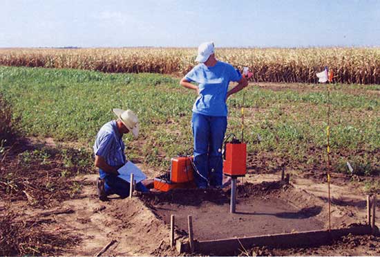
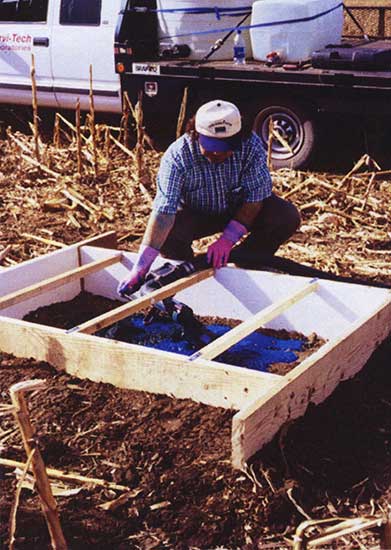
Aluminized steel pipe of 2.05-inch OD and 1.85-inch ID was used for the neutron probe access tube. A solid steel point was welded in the lower end of the pipe, as shown in Fig. 3. The neutron probe was calibrated in the field as follows. A 2.25-inch diameter, 50-ft hole was cored with the Giddings probe, and the access tube was snuggly inserted down the hole (Fig. 4). The collected core was cut in 6-inch increments, weighted in the field, and taken to the Servi-Tech, Inc. soils lab for oven-drying and re-weighing. Following access tube installation, neutron profile readings were taken in 6-inch increments within the root zone (6-ft) and in 1-ft increments from the bottom of the root zone to 50 ft. At each site, two field corner (6-by 6-ft) plots were selected as additional calibration plots in which a 10-ft access was install in each. One plot was used for the neutron moisture calibration at the dry end-end of the moisture range, whereas the other plot was periodically wetted by applying measured amounts of water for neutron probe calibration at the wet end of the moisture range. Figure 5 shows the "wet" plot with the neutron probe being used for calibration measurements. Periodically, 8-ft long cores were collected from within the corner, calibration plots with the Giddings probe, and moisture content was calculated by oven-drying for comparison with neutron readings.
Figure 3--Aluminized steel pipe and solid steel point employed in the construction of the neutron probe access tube.
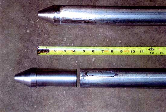
Figure 4-Field installation and welding of the neutron access tube.
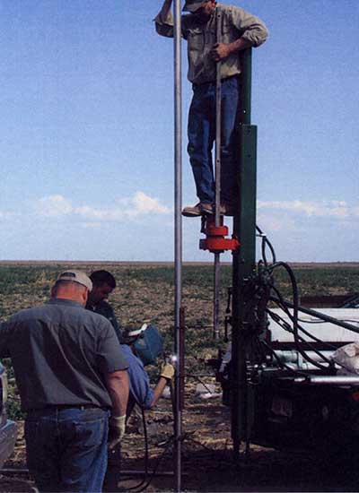
Figure 5-Field corner "wet" plot for neutron probe calibration.
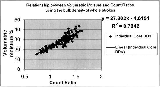
To convert gravimetric to volumetric moisture content, three methods were employed to estimate the soil bulk density with which the gravimetric water content was multiplied to obtain the volumetric water content: (1) the 6-inch core increments of known volume (4.0-cm in diameter) were weighted in the field and oven-dried in the lab; (2) the 4-ft Giddings probe stroke was measured for its collected core length and the weights of all the 6-inch core increments were added together to obtain the 4-ft stroke bulk density; (3) an average of three consecutive 6-inch core samples was obtained for a smother bulk density profile estimation. The last method of three-sample averaging was finally adopted as giving the most consistent results. Since both R8 and N7 sites have similar soils, all data from both the deep access tubes and the corner plots were combined to obtain the calibration curve shown in figure 6.
Figure 6--Neutron probe calibration curve.
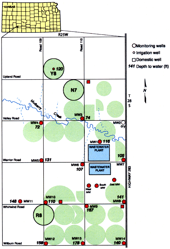
We also sampled most of the existing wells in the area (Fig. 7) to check any impacts on the relatively deep water table, which ranges from about 70-ft close to Mulberry Creek to more than 150-ft deep as one goes away from Mulberry Creek. Water samples from monitoring, domestic, and irrigation wells and wastewater lagoons were collected by both KGS and OMI personnel.
Figure 7--Depth to water measured in monitoring wells at study site in the fall of 2005.
Samples collected from domestic and irrigation wells by KGS personnel were pumped for a minimum of 10 minutes with the specific conductance and temperature being measured until both had stabilized over a sequence of three measurements. Samples were collected and kept on ice until returned to the KGS laboratory. Samples were kept in a refrigerator until analyzed. Samples for isotope analysis were kept frozen, then sent on ice to the University of Virginia laboratory for analysis and kept frozen until analyzed.
Complete inorganic water analyses were performed by the Analytical Services Section, Kansas Geological Survey (KGS). Samples for nitrate-N analysis were collected in 250-ml bottles treated with 2-ml of 10% HCl acid for preservation. Samples for all other inorganic constituents were collected in acid-rinsed 1-L polyethylene bottles, with 1-L bottles used for nitrogen-15 analyses. If needed, samples were filtered in the laboratory using a 45µ Micropore© filter prior to chemical analysis. Samples were analyzed for major cations (calcium, magnesium, sodium, potassium) and anions (chloride, bicarbonate, sulfate, nitrate, and fluoride), and other minor constituents, in addition to pH, specific conductance, temperature, and calculated total dissolved solids using standard methods described by Hathaway et al. (1975). Nitrate-N was determined using a UV method developed at the KGS (Hathaway, 1990).
Samples from the wastewater lagoons were collected by OMI personnel and analyzed by Servi-Tech labs for complete analyses (http://devteam.greensoft.com/ServitechLab/Portals/O/feeschedule.pdf).
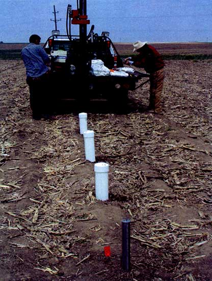
Suction lysimeters were installed at three depth levels using the Servi-Tech Giddings soil auger rig: shallow (5-6 ft), intermediate (17-26 ft), and deep (30 to 50 ft) in all sites for complete water analyses, periodic measurements of nitrate and chloride levels in pore waters, and isotopic analysis. Figure 8 shows the three depth lysimeters with PVC covers and the neutron access tube in the foreground.
Figure 8--Multi-level suction lysimeters (covered with white PVC pipe) and neutron access tube (foreground).
In order to determine the preferential flow potential of each of the two major soil types in the study area in which we established our study sites (site R8 in Harney soil, and site N7 in Ulysses soil) and better explain the deep occurrences of nitrogen concentrations, we conducted two dye-tracer experiments. A literature search for a suitable dye tracer (Flury and Fluhler, 1994a,b; 1995, Petersen et al., 1997, Schwartz et al., 1999, Flury and Wai, 2003) revealed that the brilliant blue food coloring dye (FD&C Blue 1, tri-phenyl-methane dye) would be a suitable tracer because of its desirable properties of mobility and distinguishability in soils, and also nontoxicity. In June 2005 we conducted an initial pilot tracer dye solution experiment at the KGS experimental site (GEMS) in Lawrence, KS, to check on dye effectiveness in visualizing flow patterns in soils. That test proved successful and thus we decided to proceed with the brilliant blue dye tracer experiments at the study sites following the harvesting of corn that was planted at the sites. These experiments were finally conducted on November 8, 2005, following a number of postponements due to weather problems.
The steps we followed in conducting the dye-tracer tests at sites R8 and N7 are as follows: We rented a lOOO-gallon water tank and filled it with 400 gallons of water. We then added a carefully pre-weighted total quantity of 6,056.7 grams of brilliant blue powder dye (3,028.4 grams per 200 gallons of water) and mixed it well to obtain a dye concentration of 4 g/L (which was also employed in the studies cited above). We prepared two 3' x 5' wooden rectangular frames of 1-ft height for flooding the sites with the dye solution as shown in fig. 9.
Figure 9--Wooden rectangular frame for flooding the site with dye solution.
The amount of brilliant blue dye required to arrive at a concentration of 4 g/L was arrived as follows: The 3' x 5' wooden enclosure we set up at each site would allow flooding of a 15-square foot area. Assuming an average soil porosity (based on neutron soil moisture profile readings) of 30%, the volume of solution needed to saturate the 15-ft2 area down to a depth of approximately 5 ft would be 22.5 ft3 or 168.3 gallons, and thus to achieve the desired dye concentration of 4 g/L, we would need to add 2,548.8 g of brilliant blue powder dye to that volume. However, because it would be rather difficult to accurately measure such an odd quantity of 168.3 gallons in a water tank, we decided to re-compute the weight of needed powder dye for a round-number volume of 200 gallons of water. Thus, to come up with the desired concentration of 4 g/L, we would need 3,028.4 g of dye in 200 gal of water.
The USDA-ARS developed a Root Zone Water Quality Model (RZWQM), which includes a submodel for macropore flow and transport, as well as other modules for pesticide reactions and degradations, nutrient transformations, plant growth, and management-practice effects. One of the objectives of this study is to use the RZWQM model to study magnitudes and characteristics of macropore flow and transport as influenced by important factors in the typical soils of the area.
The Root Zone Water Quality Model (RZWQM) is a one-dimensional (vertical in the soil profile) process-based model (Ahuja et al., 2000) that simulates the growth of the plant and the movement of water, nutrients, and agro-chemicals over, within, and below the crop root zone of a unit area of an agricultural cropping system under a range of common management practices. It uses the Green-Ampt equation to simulate infiltration and Richards equation to simulate water redistribution. Rainfall or irrigation water in excess of the soil-infiltration capacity (overland flow) is routed into macropores if present. The maximum macropore flow rate and lateral water movement into macropores in the surrounding soil are computed using Poiseuilles' law and the lateral Green-Ampt equation. Macropore flow in excess of its maximum flow rate or excess infiltration is routed to runoff.
The nutrient sub-model for organic matter/nitrogen cycling of RZWQM simulates all the major pathways including mineralization-immobilization of crop residues, manure, and other organic wastes; mineralization of the soil humus fractions; inter-pool transfers of carbon and nitrogen; denitrification (production of N2 and N2O); gaseous loss of ammonia (NH3); nitrification of ammonium to produce nitrate- N; production and consumption of methane gas (CH4) and carbon dioxide (CO2); and microbial biomass growth and death. Despite the complexity of this organic matter/N-cycling component, good estimates of initial soil carbon content and nitrogen are generally the only site-specific parameters needed. The required inputs (e.g. fast pool, slow pool) are then usually determined through an initiation wizard and calibration.
We will investigate whether significant preferential flow is occurring and determine the prediction errors made in terms of soil moisture and N-concentrations when preferential flow is ignored. Parameters for soil-hydraulic properties in the model to be employed will be measured, taken from the literature, calibrated, or estimated from soil texture, soil structure, bulk density, and organic carbon content using pedo-transfer functions.
(The information in this section was adapted from the on-line documentations of the RETC and ROSETTA programs from the Agricultural Research Service, US Department of Agriculture web site at http://www.ars.usda.gov/Services/docs.htm?docid=8952&pf=1 and http://www.ars.usda.gov/Services/docs.htm?docid=8953.)
Most vadose zone studies today use numerical models to simulate the movement of water and solutes in the subsurface. Knowledge about the soil hydraulic properties (i.e., the water retention curve and hydraulic conductivity) is essential for running these models. A broad array of methods currently exists to determine soil hydraulic properties in the field or in the laboratory (cf. Klute, 1986; van Genuchten et at, 1992). Most laboratory and field techniques, however, have specific ranges of applicability with respect to soil type and saturation (Klute, 1986). In addition, measurements of the soil hydraulic conductivity and/or soil water retention curve are costly, time consuming, and sometimes unreliable because of soil heterogeneity and experimental errors.
A large number of indirect methods to generate soil hydraulic properties are now available. Although these methods vary widely in terms of methodology and complexity, all use some form of surrogate data to estimate soil hydraulic properties. In broad terms, three methods can be distinguished; pore-size distribution or parametric models, inverse methods, and pedotransfer functions. We will address the first and last methods here.
Pore-size distribution models or parametric models for the soil hydraulic functions are very often used to estimate the unsaturated hydraulic conductivity from the distribution, connectivity and tortuosity of pores. The pore-size distribution can be inferred from the water retention curve, which is normally much easier to measure than the unsaturated hydraulic conductivity function. One of the most popular models was developed by Mualem (1976). The model may be simplified into closed-form expressions when the water retention is described with the functions of Brooks-Corey (1964) or van Genuchten (1980). The RETC (RETention Curve) computer program for describing the hydraulic properties of unsaturated soils may be used to fit several such analytical models to observed water retention and/or unsaturated hydraulic conductivity data.
Parametric Models for the Soil Hydraulic Function: Water flow in variably-saturated soils is traditionally described with the Richards equation
C (δψ / δt) = (δ/δz) [K δψ / δt - K] (1)
where ψ is the soil water pressure head (with dimension L), t is time (T), z is soil depth (L), K is the hydraulic conductivity (LT-1), and C is the soil water capacity (L-1) approximately by the slope (dθ/dψ) of the soil water retention curve, θ(ψ), in which θ is the volumetric water content (L3L-3). The solution of the Richards equation requires knowledge of the unsaturated soil hydraulic functions θ(ψ) and K(ψ) or K(θ).
One of the most popular functions for describing the θ(ψ) function has been the equation of Brooks and Corey (1964), further referred to as the BC-equation:
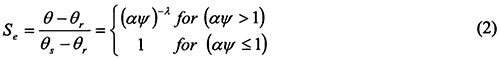
where Se is the effective degree of saturation, also called the reduced water content (0 ≤ Se ≤ 1), θr and θs are the residual and saturated water contents, respectively; α is an empirical parameter (L-1) whose inverse is often referred to as the air entry value or bubbling pressure, and λ is a poresize distribution parameter affecting the slope of the retention function. For notational convenience, ψ and α are taken positive for unsaturated soils (i.e., ψ denotes suction).
Several continuously differentiable (smooth) equations have been proposed to improve the description of soil water retention near saturation. A related smooth function with attractive properties is the equation of van Genuchten [1980], further referred to as the VG-equation:
Se = [1 + (αψ)n]m (3)
where α(L-2), n and m are empirical constants affecting the shape of the retention curve, and m is normally calculated as m = 1-1/n.
The corresponding closed-form expression for the unsaturated hydraulic conductivity, K (e.g., cm/day), is (van Genuchten, 1980):
K(Se) = KoSeL {1 - [1- Sen/(n-1)]1-1/n}2 (4)
in which Ko is a matching point at saturation (cm/day) and similar, but not necessarily equal, to the saturated hydraulic conductivity, K; The parameter L (-) is an empirical pore tortuosity/connectivity parameter that is normally assumed to be 0.5 (Mualem, 1976).
Pedotranfer functions (PTFs, Bouma and van Lanen, 1987) offer another method for estimating hydraulic properties by using the fact that hydraulic properties are dependent upon soil texture and other readily available taxonomic information (e.g., the particle size distribution, bulk density and/or organic matter content). For example, fine-textured soils are known to have very different water retention characteristics and much lower saturated hydraulic conductivities than coarse-textured soils. PTFs take advantage of such information. Although considerable differences exist among PTFs in terms of the required input data (Rawls et al., 1992), all of them use at least some information about the particle-size distribution.
The computer model ROSETTA implements PTFs to predict van Genuchten (1980) water retention parameters and saturated hydraulic conductivity (Ks) by using textural class, textural distribution, bulk density and one or two water retention points as input. Although the use of more input data often leads to better predictions (Schaap and Bouten, 1996; Schaap et al., 1998) there are many cases where only limited soil information is available. ROSETTA follows a hierarchical approach to estimate water retention and Ks values using limited or more extended sets of input data (Schaap et al., 1998, Schaap and Leij, 1998a).
The hierarchical approach is reflected in the five models employed in ROSETTA. The simplest model consists of a lookup table for average hydraulic parameters for each soil textural class (sand, silty loam, clay loam, etc.). The other four models are based on neural network analysis (Schaap et al., 1998) and predict the hydraulic parameters, using additional input variables, with an increasing degree of accuracy. All five models haven been calibrated on the same data set and provide consistent predictions. The calibration data set contained 2,134 samples for water retention and 1,306 samples for saturated hydraulic conductivity, Ks (Schaap and Leij, 1998b). The samples were obtained from a large number of sources and involve agricultural and non-agricultural soils in temperate climate zones of the northern hemisphere (mainly from the USA and some from Europe). The output from the ROSETTA program provides for the θr, θs, the van Genuchten parameters α and n, and Ks values.
Splus 7.0 for Windows was used for statistical evaluation of water samples. The tests used were from the environmental statistics module developed by Millard (2002). The Shapiro-Wilk test was used to determine if the evaluated parameters were normally distributed. The test showed that the parameters evaluated (nitrate-N, chloride, specific conductance, and sulfate) were not normal so nonparametric tests were used for the hypothesis testing. The Kruskal-Wallis test was used for hypothesis testing for homogeneity of variances (do the values belong in the same group or are they different). The method used the Levene test for homogeneity of variance.
The soils at all sites were described from collected cores by NRCS scientists. The soils belong to the Harney-Ulysses silt loam/silty clay loam series family and are described in detail in Appendix A. Textural and other analyses of the top 5.4 m of site R8 and the top 12.2 m of site N7 as determined at the NRCS Soil Survey Lab in Lincoln, Nebraska are shown in Table 1, and the corresponding analyses of the top 0.5 m of site Y8 as determined by the KSU Soil Testing Lab are shown in Table 2.
Concentrations of total carbon (Ctot) and carbonates (CaCO3) are also shown in Tables 1 and 2 for all sites. Total carbon is the sum of organic and inorganic carbon. Most of the organic carbon is associated with the organic matter fraction and the inorganic carbon is generally found with carbonate minerals.
One of the most important interactions in soils is cation exchange, in which positively charged ions are attracted to the negatively charged surfaces of clays and organic matter where they are loosely held. These cations are a major source of plant nutrients. Tables 1 and 2 contain the CEC and/or SAR for the soils at R8, N7, and Y8 sites.
The soil bulk density down to 15.2 m (50 ft) was determined from collected cores of known diameter by cutting the core in 15.2-cm (6-in) increments, weighing them in the field, and then oven-drying them in the lab. The data were smoothed by taking the average of three 15-cm samples and displayed in figure 10 for sites R8 and N7.
Sites R8 and N7 have been planted with corn in April 2005 and harvested in September 2005. Site N7 has been in corn since 1998, whereas site R8 since 2003, although it has also been planted with corn in 1996.
Figure 10--Soil bulk density profiles.
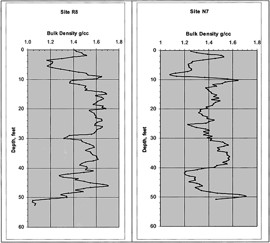
Table 1--Soil horizon textural and total Carbon (Ctot) and carbonate (CaCO3) analyses for sites R8 and N7 from NRCS
| Site | layer_seq | hzn_top (cm) |
hzn_bot (cm) |
hzn | texture | Clay (%) |
Silt (%) |
Sand (%) |
Ctot (%) |
CaCO3 (%) |
CEC (cmol(+)/kg) |
SAR (%) |
|---|---|---|---|---|---|---|---|---|---|---|---|---|
| R8 | 1 | 0 | 16 | Ap | Silt loam | 31.6 | 64.3 | 4.1 | 1.66 | tr | 23 | 2 |
| R8 | 2 | 16 | 29 | Bt1 | Silty clay loam | 30.5 | 65.9 | 3.6 | 1.03 | tr | 20.8 | 5 |
| R8 | 3 | 29 | 50 | Bt2 | Silty clay loam | 37.8 | 59.9 | 2.3 | 0.75 | tr | 25.6 | 6 |
| R8 | 4 | 50 | 68 | Bt3 | Silty clay loam | 43 | 55.3 | 1.7 | 0.56 | tr | 30.4 | 6 |
| R8 | 5 | 68 | 90 | Btk | Silty clay loam | 38.7 | 59.2 | 2.1 | 0.66 | 2 | 27.5 | 6 |
| R8 | 6 | 90 | 140 | Btk2 | Silty clay loam | 34.3 | 62.7 | 3 | 1.06 | 6 | 23.8 | 6 |
| R8 | 7 | 140 | 185 | Btk3 | Silty clay loam | 33.3 | 61.5 | 5.2 | 0.63 | 3 | 22.6 | 6 |
| R8 | 8 | 185 | 260 | Btk4 | Silty clay loam | 34.6 | 50.2 | 15.2 | 2.45 | 19 | 16 | 4 |
| R8 | 9 | 260 | 300 | 2Btk5 | Silty clay loam | 32.3 | 48.3 | 19.4 | 17 | 16.3 | 3 | |
| R8 | 10 | 300 | 410 | 2Btk6 | Silty clay loam | 28.9 | 49.4 | 21.7 | 1.28 | 11 | 16 | 3 |
| R8 | 11 | 410 | 485 | 2Btk7 | Silty clay loam | 31.6 | 49.6 | 18.8 | 1.67 | 14 | 17.5 | 2 |
| R8 | 12 | 485 | 540 | 2Bk | Silty clay loam | 39.9 | 49.7 | 10.4 | 4.76 | 37 | 12.8 | 1 |
| N7 | 1 | 0 | 13 | Ap | Silt loam | 24.2 | 68.3 | 7.5 | 1.53 | tr | 19.3 | 3 |
| N7 | 2 | 13 | 23 | A | Silt loam | 27.4 | 68.9 | 3.7 | 1.06 | tr | 20.2 | 4 |
| N7 | 3 | 23 | 43 | Bt1 | Silt loam | 31.3 | 66 | 2.7 | 0.78 | tr | 21.5 | 5 |
| N7 | 4 | 43 | 74 | Bt2 | Silty clay loam | 39.1 | 58.2 | 2.7 | 0.53 | tr | 27.5 | 5 |
| N7 | 5 | 74 | 91 | Btk | Silty clay loam | 38.4 | 59.9 | 1.7 | 0.71 | 3 | 27.4 | 4 |
| N7 | 6 | 91 | 119 | Bk1 | Silty clay loam | 32.9 | 64 | 3.1 | 1.31 | 9 | 22.8 | 3 |
| N7 | 7 | 119 | 168 | Bk2 | Silt loam | 31.8 | 63.2 | 5 | 0.62 | 3 | 22.4 | 1 |
| N7 | 8 | 168 | 221 | Bw | Loam | 32.8 | 55.8 | 11.4 | 1.32 | 9 | 18.7 | 2 |
| N7 | 9 | 221 | 295 | BCk1 | Silty clay loam | 33.3 | 51.6 | 15.1 | 2.29 | 19 | 14.6 | 4 |
| N7 | 10 | 295 | 363 | BCk2 | Silty clay loam | 3.93 | 31 | 12 | 4 | |||
| N7 | 11 | 363 | 399 | Bkb1 | Silty clay loam | 32.9 | 59.2 | 7.9 | 2.83 | 23 | 14.3 | 4 |
| N7 | 12 | 399 | 467 | Bkb2 | Silty clay loam | 27.7 | 63.1 | 9.2 | 1.19 | 10 | 15.2 | 3 |
| N7 | 13 | 467 | 508 | C1 | Loam | 2.04 | 17 | 14.1 | 3 | |||
| N7 | 14 | 508 | 625 | C2 | Silty clay loam | 29.3 | 60.9 | 9.8 | 0.83 | 7 | 18.9 | 2 |
| N7 | 15 | 625 | 762 | C3 | Silt loam | 26.6 | 62.4 | 11 | 2.46 | 20 | 12.1 | 2 |
| N7 | 16 | 762 | 848 | C4 | Silt loam | 22.1 | 63.8 | 14.1 | 1.58 | 13 | 13.1 | 2 |
| N7 | 17 | 848 | 889 | C5 | Silt loam | 0.75 | 6 | 16.9 | 1 | |||
| N7 | 18 | 889 | 945 | C6 | Loam | 22 | 51.3 | 26.7 | 1.03 | 9 | 12.7 | 1 |
| N7 | 19 | 945 | 1016 | C7 | Loam | 21 | 40 | 39 | 1.14 | 10 | 10.6 | 1 |
| N7 | 20 | 1016 | 1080 | C8 | Loam | 27.2 | 43.1 | 29.7 | 0.88 | 7 | 15.7 | 1 |
| N7 | 21 | 1080 | 1118 | C9 | Loam | 26 | 35.9 | 38.1 | 2.42 | 20 | 10.6 | 1 |
| N7 | 22 | 1118 | 1148 | C10 | Loam | 23.4 | 44.4 | 32.2 | 0.62 | 5 | 13.5 | |
| N7 | 23 | 1148 | 1219 | C11 | Loam | 18 | 29 | 53 | 1.85 | 15 | 8.2 |
Table 2--Soil horizon textural and total Carbon (Ctot) and carbonate (CaCO3) analyses for site Y8 from KSU.
| Site | layer | depth from (cm) |
depth to (cm) |
clay (%) |
silt (%) |
sand (%) |
Ctot (%) |
CaCO3 (%) |
CEC (meq/100g) |
|---|---|---|---|---|---|---|---|---|---|
| Y8 | 1 | 0 | 15.24 | 22 | 56 | 22 | 1.20 | 0.0 | 14.2 |
| Y8 | 2 | 15.24 | 30.48 | 26 | 52 | 22 | 0.78 | 0.0 | 16.4 |
| Y8 | 3 | 30.48 | 45.72 | 30 | 52 | 18 | 0.57 | 0.0 | 15.2 |
| Y8 | 4 | 45.72 | 60.96 | 40 | 44 | 16 | 0.61 | 0.1 | 19.9 |
| Y8 | 5 | 60.96 | 76.2 | 40 | 46 | 14 | 0.59 | 1.2 | 22.1 |
| Y8 | 6 | 76.2 | 91.44 | 38 | 48 | 14 | 0.62 | 1.2 | 22.5 |
| Y8 | 7 | 91.44 | 106.7 | 38 | 48 | 14 | 0.57 | 1.2 | 18.9 |
| Y8 | 8 | 106.7 | 121.9 | 36 | 50 | 14 | 0.47 | 1.1 | 21.6 |
| Y8 | 9 | 121.9 | 137.2 | 34 | 50 | 16 | 0.42 | 1.1 | 19.9 |
| Y8 | 10 | 137.2 | 152.4 | 34 | 52 | 14 | 0.30 | 0.6 | 16.0 |
| Y8 | 11 | 152.4 | 167.6 | 30 | 54 | 16 | 0.22 | 0.8 | 15.8 |
| Y8 | 12 | 167.6 | 182.9 | 28 | 54 | 18 | 0.21 | 0.9 | 14.9 |
| Y8 | 13 | 182.9 | 198.1 | 28 | 54 | 18 | 0.24 | 0.5 | 15.1 |
| Y8 | 14 | 198.1 | 213.4 | 30 | 50 | 20 | 0.29 | 0.2 | 13.3 |
| Y8 | 15 | 213.4 | 228.6 | 30 | 54 | 16 | 0.26 | 0.3 | 23.3 |
| Y8 | 16 | 228.6 | 243.8 | 30 | 54 | 16 | 0.33 | 0.2 | 8.6 |
| Y8 | 17 | 243.8 | 259.1 | 30 | 50 | 20 | 0.44 | 0.0 | 13.3 |
| Y8 | 18 | 259.1 | 274.3 | 30 | 48 | 22 | 0.39 | 0.0 | 13.0 |
| Y8 | 19 | 274.3 | 289.6 | 34 | 40 | 26 | 0.27 | 14.0 | 11.9 |
| Y8 | 20 | 289.6 | 304.8 | 40 | 34 | 26 | 0.19 | 33.6 | 9.8 |
The saturated hydraulic conductivity was determined on collected 5.08-cm (2-in) core from sites R8 and N7 according to ASTM-D5084 Flexible wall permeameter test. The samples were classified according to the Unified Soil Classification System as fine-grained, medium to high plasticity lean clay and fat clay (CL and CH)-soils. Table 3 shows the analysed core intervals, the soil Unified Classification, the measured bulk density, and the resulting saturated hydraulic conductivity.
Table 3--Saturated hydraulic conductivity from collected cores.
| Site | Depth (cm) |
Unified Classification |
Bulk Density (g/cc) |
Hydraulic conductivity (cm/sec) |
|---|---|---|---|---|
| R8 | 0-16 | CL | 1.38 | 1.4x10⁻⁶ |
| R8 | 16-29 | CL | 1.42 | 2.4x10⁻⁷ |
| R8 | 29-50 | CH | 1.39 | 4.3x10⁻⁷ |
| R8 | 50-68 | CH | 1.49 | 3.2x10⁻⁶ |
| R8 | 68-90 | CH | 1.45 | 1.4x10⁻⁴ |
| R8 | 90-140 | CL | 5.2x10⁻⁵ | |
| R8 | 410-485 | CL | 1.64 | 4.2x10⁻⁶ |
| N7 | 15-30 | CL | 1.19 | 1.5x10⁻⁵ |
| N7 | 30-61 | CL | 1.32 | 2.0x10⁻⁵ |
| N7 | 61-91 | CH | 1.26 | 6.3x10⁻⁶ |
| N7 | 91-122 | CL | 1.36 | 6.8x10⁻⁴ |
| N7 | 152-183 | CL | 1.36 | 5.6x10⁻⁵ |
| N7 | 183-213 | CL | 1.42 | 4.5x10⁻⁶ |
| N7 | 305-335 | CL | 1.52 | 9.3x10⁻⁶ |
| N7 | 457-488 | CL | 1.50 | 5.2x10⁻⁴ |
The gravimetric water content data corresponding to seven applied pressures (0.06, 0.10, 0.33, 1,2,5, and 15 bar) for collected samples from sites R8 and N7 are presented in Table 4 from the NRCS Soil Survey Lab. Water retention at 0.06 to 5 bar were determined by pressure-plate extraction, whereas at 15 bar by pressure-membrane extraction.
Table 4--Water retention data (i.e., gravimetric water content {%} at different pressures {bar}) for sites R8 and N7 from NRCS lab analyses
| Site | hzn_top (cm) |
hzn_bot (cm) |
hzn | texture | 0.06 bar (%) |
0.10 bar (%) |
0.33 bar (%) |
1 bar (%) |
2 bar (%) |
5 bar (%) |
15 bar (%) |
|---|---|---|---|---|---|---|---|---|---|---|---|
| R8 | 0 | 16 | Ap | Silt loam | 47.3 | 43.3 | 35.4 | 23.4 | 18.6 | 16.9 | 15 |
| R8 | 16 | 29 | Bt1 | Silty clay loam | 45.3 | 41.9 | 35.3 | 23.4 | 17.9 | 16.3 | 14.2 |
| R8 | 29 | 50 | Bt2 | Silty clay loam | 48 | 43.8 | 38 | 27.5 | 22.4 | 20.3 | 17.8 |
| R8 | 50 | 68 | Bt3 | Silty clay loam | 49.8 | 45.1 | 39.5 | 31.1 | 25.9 | 23.8 | 20.1 |
| R8 | 68 | 90 | Btk | Silty clay loam | 47.9 | 43.4 | 38.2 | 29.5 | 24.3 | 23.3 | 21.7 |
| R8 | 90 | 140 | Btk2 | Silty clay loam | 48.8 | 43.4 | 36.6 | 26.7 | 23 | 20.7 | 16.7 |
| R8 | 140 | 185 | Btk3 | Silty clay loam | 47 | 42.1 | 36.9 | 26.4 | 22.5 | 20 | 14.9 |
| R8 | 185 | 260 | Btk4 | Silty clay loam | 40.2 | 35.8 | 29.9 | 22.2 | 19.2 | 17.4 | 13.1 |
| R8 | 260 | 300 | 2Btk5 | Silty clay loam | 36.3 | 34 | 28 | 21 | 18.2 | 16.8 | 12.6 |
| R8 | 300 | 410 | 2Btk6 | Silty clay loam | 36.5 | 34 | 27.3 | 20.3 | 17.3 | 16.2 | 11.9 |
| R8 | 410 | 485 | 2Btk7 | Silty clay loam | 36.5 | 33.7 | 29.2 | 22 | 19.2 | 17.7 | 12.8 |
| R8 | 485 | 540 | 2Bk | Silty clay loam | 35.3 | 30.6 | 26.6 | 20.6 | 19.4 | 17.7 | 12.7 |
| N7 | 0 | 13 | Ap | Silt loam | 20.4 | 17.6 | 15.1 | 13 | |||
| N7 | 13 | 23 | A | Silt loam | 20.6 | 18.3 | 15.8 | 13.1 | |||
| N7 | 23 | 43 | Bt1 | Silt loam | 22.7 | 20.2 | 18.3 | 15.1 | |||
| N7 | 43 | 74 | Bt2 | Silty clay loam | 28.4 | 25.5 | 23.6 | 18.7 | |||
| N7 | 74 | 91 | Btk | Silty clay loam | 28.1 | 25.4 | 23.5 | 18.2 | |||
| N7 | 91 | 119 | Bk1 | Silty clay loam | 25.9 | 22.7 | 20.2 | 15.6 | |||
| N7 | 119 | 168 | Bk2 | Silt loam | 24.1 | 21 | 18.5 | 14.7 | |||
| N7 | 168 | 221 | Bw | Loam | 21.4 | 19.1 | 16.9 | 14.1 | |||
| N7 | 221 | 295 | BCk1 | Silty clay loam | 18.8 | 16.6 | 15.3 | 12.1 | |||
| N7 | 295 | 363 | BCk2 | Silty clay loam | 20.8 | 18.2 | 16.5 | 12.2 | |||
| N7 | 363 | 399 | Bkb1 | Silty clay loam | 20.7 | 19 | 16.3 | 12.3 | |||
| N7 | 399 | 467 | Bkb2 | Silty clay loam | 21.2 | 16.4 | 14.8 | 11.3 | |||
| N7 | 467 | 508 | C1 | Loam | 20.8 | 16.7 | 15 | 11.3 | |||
| N7 | 508 | 625 | C2 | Silty clay loam | 22.7 | 17.7 | 15.9 | 12.5 | |||
| N7 | 625 | 762 | C3 | Silt loam | 21.3 | 16.7 | 14.7 | 11.2 | |||
| N7 | 762 | 848 | C4 | Silt loam | 18.4 | 14.4 | 12.7 | 10.2 | |||
| N7 | 848 | 889 | C5 | Silt loam | 22.3 | 17.4 | 15.6 | 12.6 | |||
| N7 | 889 | 945 | C6 | Loam | 17.3 | 13.7 | 12.3 | 9.6 | |||
| N7 | 945 | 1016 | C7 | Loam | 15.6 | 12.4 | 10.9 | 8.7 | |||
| N7 | 1016 | 1080 | C8 | Loam | 20.7 | 16.8 | 14.8 | 11.6 | |||
| N7 | 1080 | 1118 | C9 | Loam | 16.5 | 13.6 | 11.9 | 9.6 | |||
| N7 | 1118 | 1148 | C10 | Loam | 17.6 | 13.8 | 12.4 | 10.2 | |||
| N7 | 1148 | 1219 | C11 | Loam | 12.6 | 9.8 | 8.8 | 6.9 | |||
| N7 core | 0 | 30 | 22.6 | ||||||||
| N7 core | 30 | 61 | 23.3 | ||||||||
| N7 core | 61 | 91 | 25.4 | ||||||||
| N7 core | 91 | 122 | 27.3 | ||||||||
| N7 core | 122 | 152 | 28.3 | ||||||||
| N7 core | 152 | 183 | 27.1 | ||||||||
| N7 core | 183 | 213 | 23.9 | ||||||||
| N7 core | 305 | 335 | 20.7 | ||||||||
| N7 core | 457 | 488 | 22.8 | ||||||||
| N7 core | 609 | 640 | 23.4 | ||||||||
| N7 core | 914 | 945 | 24.8 |
The RETC-estimated Brooks and Corey (BC) parameters (α and λ) and the ROSETTA-estimated Van Genuchten parameters (α and n) and Ks values for the samples displayed in Table 1 are shown in Table 5. For the RETC program, we input as θr the estimates predicted by ROSETTA, and as θs the porosity values calculated by the equation
φ = 1 - (ρb / ρs) (5)
where φ is the soil porosity (equal to θs), ρb is the soil bulk density (taken from Fig. 5), and ρs is the particle density, taken as that for quartz (2.65 g/cc). We then used the RETC parameter estimation program to optimize for θs, α, and λ (for the BC parameters) keeping the θr values fixed as estimated from ROSETTA.
Please note that because some of the NRCS lab-determined moisture values corresponding to various pressures for site R8 were higher than the values of porosity determined by eq. (5) above, the lab-determined moisture values corresponding to the various pressures were scaled as follows:
θi =(θi / θi-1) * θi-1 (6)
where the subscript i (taking the successive values of 0.10, 0.33, 1, 2, and 15 bar) refers to the applied pressure for the corresponding moisture, and the moisture content corresponding to the initially applied pressure of 0.06 bar was taken as equal to θs.
Table 5--Brooks and Corey- and Rosetta-estimated Van Genuchten hydraulic parameters for soil samples from sites R8 and N7.
| Site | hzn_top (cm) |
hzn_bot (cm) |
hzn | texture | RETC: Brooks and Corey | ROSETTA | |||||||
|---|---|---|---|---|---|---|---|---|---|---|---|---|---|
| Theta-R (-) |
Theta-S (-) |
alpha (1/cm) |
lambda (-) |
Theta-R (-) |
Theta-S (-) |
alpha (1/cm) |
n (-) |
Ks (cm/day) |
|||||
| R8 | 0 | 16 | Ap | Silt loam Silty clay |
0.0692 | 0.4463 | 0.0105 | 0.3329 | 0.0692 | 0.4461 | 0.0034 | 1.6051 | 10.7523 |
| R8 | 16 | 29 | Bt1 | Loam Silty clay |
0.0660 | 0.4216 | 0.0056 | 0.4423 | 0.066 | 0.4396 | 0.0033 | 1.6338 | 10.9245 |
| R8 | 29 | 50 | Bt2 | Loam Silty clay |
0.0850 | 0.4928 | 0.0064 | 0.3384 | 0.085 | 0.4667 | 0.0019 | 1.6726 | 3.6787 |
| R8 | 50 | 68 | Bt3 | Loam Silty clay |
0.0866 | 0.5182 | 0.0112 | 0.2258 | 0.0866 | 0.4745 | 0.0017 | 1.6092 | 2.1370 |
| R8 | 68 | 90 | Btk | Loam Silty clay |
0.0874 | 0.5002 | 0.0119 | 0.2159 | 0.0874 | 0.4897 | 0.0041 | 1.4041 | 6.7174 |
| R8 | 90 | 140 | Btk2 | Loam Silty clay |
0.0650 | 0.4280 | 0.0148 | 0.2710 | 0.065 | 0.4746 | 0.0080 | 1.4474 | 20.4033 |
| R8 | 140 | 185 | Btk3 | Loam Silty clay |
0.0648 | 0.4343 | 0.0133 | 0.2742 | 0.0648 | 0.4821 | 0.0050 | 1.5563 | 25.4097 |
| R8 | 185 | 260 | Btk4 | Loam Silty clay |
0.0538 | 0.4049 | 0.0190 | 0.2607 | 0.0538 | 0.4007 | 0.0067 | 1.4415 | 7.7678 |
| R8 | 260 | 300 | 2Btk5 | Loam Silty clay |
0.0530 | 0.3806 | 0.0076 | 0.2966 | 0.053 | 0.3814 | 0.0049 | 1.4511 | 3.7034 |
| R8 | 300 | 410 | 2Btk6 | Loam Silty clay |
0.0565 | 0.4231 | 0.0091 | 0.3152 | 0.0565 | 0.4061 | 0.0046 | 1.5028 | 7.1236 |
| R8 | 410 | 485 | 2Btk7 | Loam Silty clay |
0.0592 | 0.4380 | 0.0153 | 0.2453 | 0.0592 | 0.3986 | 0.0031 | 1.5499 | 3.1391 |
| R8 | 485 | 540 | 2Bk | Loam | 0.0852 | 0.5897 | 0.0220 | 0.1764 | 0.0852 | 0.4074 | 0.0109 | 1.3772 | 2.6577 |
| N7 | 0 | 13 | Ap | Silt loam | 0.069 | 0.4721 | 0.0448 | 0.212 | 0.069 | 0.4554 | 0.0239 | 1.3234 | 36.6775 |
| N7 | 13 | 23 | A | Silt loam | 0.0714 | 0.4611 | 0.0313 | 0.196 | 0.0714 | 0.4547 | 0.0221 | 1.3195 | 26.5033 |
| N7 | 23 | 43 | Bt1 | Silt loam Silty clay |
0.0865 | 0.4040 | 0.0994 | 0.1722 | 0.0865 | 0.4511 | 0.0231 | 1.2560 | 15.8234 |
| N7 | 43 | 74 | Bt2 | Loam Silty clay |
0.0861 | 0.5541 | 0.0147 | 0.2033 | 0.0861 | 0.4485 | 0.0224 | 1.1639 | 2.9499 |
| N7 | 74 | 91 | Btk | Loam Silty clay |
0.081 | 0.459 | 0.0340 | 0.156 | 0.081 | 0.4675 | 0.0048 | 1.3687 | 4.5457 |
| N7 | 91 | 119 | Bk1 | Loam | 0.081 | 0.4990 | 0.0396 | 0.192 | 0.0817 | 0.4808 | 0.0110 | 1.3354 | 21.2129 |
| N7 | 119 | 168 | Bk2 | Silt loam | 0.0817 | 0.4987 | 0.008 | 0.217 | 0.0763 | 0.4845 | 0.0083 | 1.4028 | 26.5583 |
| N7 | 168 | 221 | Bw | Loam Silty clay |
0.0763 | 0.4471 | 0.0088 | 0.211 | 0.0808 | 0.4722 | 0.0245 | 1.3107 | 23.5885 |
| N7 | 221 | 295 | BCk1 | Loam Silty clay |
0.0808 | 0.5078 | 0.0236 | 0.266 | 0.0832 | 0.4227 | 0.0088 | 1.4788 | 5.4375 |
| N7 | 295 | 363 | BCk2 | Loam Silty clay |
0.0832 | 0.5282 | 0.0346 | 0.24 | |||||
| N7 | 363 | 399 | Bkb1 | Loam Silty clay |
0.0787 | 0.4632 | 0.0156 | 0.202 | 0.0787 | 0.4366 | 0.0253 | 1.2939 | 14.3814 |
| N7 | 399 | 467 | Bkb2 | Loam Silty clay |
0.0664 | 0.4483 | 0.0087 | 0.236 | 0.0664 | 0.4306 | 0.0073 | 1.3890 | 12.5112 |
| N7 | 467 | 508 | C1 | Loam | |||||||||
| N7 | 508 | 625 | C2 | Loam | 0.0548 | 0.3952 | 0.0375 | 0.2282 | 0.0548 | 0.3952 | 0.0243 | 1.3323 | 12.2096 |
| N7 | 625 | 762 | C3 | Silt loam | 0.0817 | 0.4576 | 0.0064 | 0.5641 | 0.0817 | 0.4576 | 0.0063 | 1.5926 | 17.1159 |
| N7 | 762 | 848 | C4 | Silt loam | 0.0740 | 0.4313 | 0.0056 | 0.6383 | 0.0740 | 0.4313 | 0.0056 | 1.6383 | 16.7186 |
| N7 | 848 | 889 | C5 | Silt loam | |||||||||
| N7 | 889 | 945 | C6 | Loam | 0.0563 | 0.4143 | 0.0249 | 0.3344 | 0.0563 | 0.4143 | 0.0249 | 1.3344 | 24.6093 |
| N7 | 945 | 1016 | C7 | Loam | 0.0617 | 0.3879 | 0.0102 | 0.4980 | 0.0617 | 0.3879 | 0.0102 | 1.4980 | 9.1432 |
| N7 | 1016 | 1080 | C8 | Loam | 0.0705 | 0.3878 | 0.0098 | 0.4635 | 0.0705 | 0.3878 | 0.0098 | 1.4635 | 4.9034 |
| N7 | 1080 | 1118 | C9 | Loam | 0.0662 | 0.3805 | 0.0126 | 0.4077 | 0.0662 | 0.3805 | 0.0126 | 1.4077 | 4.9682 |
| N7 | 1118 | 1148 | C10 | Loam | 0.0644 | 0.3775 | 0.0093 | 0.4880 | 0.0644 | 0.3775 | 0.0093 | 1.4880 | 5.8573 |
| N7 | 1148 | 1219 | C11 | Loam | 0.0563 | 0.3977 | 0.0166 | 0.4441 | 0.0563 | 0.3977 | 0.0166 | 1.4441 | 20.8353 |
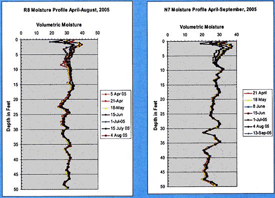
Neutron probe readings were taken twice a month during the irrigation season. Figure 11 shows neutron moisture content profiles down to 50 ft at various times during 2005 for both sites. As can be clearly seen, most of the change in soil moisture occurs in the upper 8 ft or so.
Figure 11--Soil moisture profiles at various times during 2005 measured with the neutron probe.
Following a number of weather-related delays, the dye-tracer experiments were finally conducted in November 2005. By the late morning of November 8, 2005 we initially applied approximately 90 gal of dye solution in each test site. By the late afternoon all that applied solution had infiltrated into the soil, and the 3 foot x 5 foot wooden enclosures were again filled in with dye tracer solution. The wooden frame enclosures were covered with a reflective insulating sheet and left to seep in overnight. By the next morning of November 9, 2005 nearly all the applied dye solution infiltrated in, and the remaining dye solution in the tank was applied to each site, totaling approximately 200 gallons per site. On the next morning of November 10,2005, a back-hoe was brought first to site R8 and then to site N7, where approximately 8-ft deep trenches along the diagonal of the flooded rectangular area were dug, and the dye-tracer patterns along the trench wall were observed, studied, and photographed. The trenches were covered with tarp and fenced until completion of our dye-patterns study.
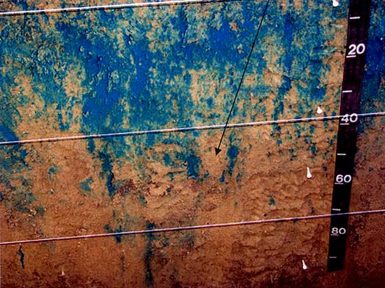
For the site R8 in Harney soil, the dye solution penetrated down to approximately 6.5 ft and formed a more-or-less uniform "finger front" at the bottom as shown in figure 12. Figure 13 shows a closer-up view of the dye tracer movement through the blocky-structure soil layers of the Bt horizons (at approximately the 1.6 to 3.2-ft depth interval) where the tracer dye moved along the spaces in-between the blocky soil aggregates and concentrated in numerous fingers in the lower soil layer that did not exhibit the heavy blocky structure of the Bt horizons above. Figure 14 shows a closer-up view of the fingers in the lower 3.2 to 6.0-ft layer, where the dye solution under tension tries to by-pass coarser-texture lenses, as shown by the arrow in the figure.
Figure 12--Uniform finger front from Brilliant Blue dye tracer experiment at site R8.
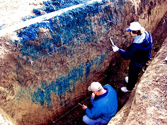
Figure 13--Brilliant Blue dye pattern detail at site R8 showing the movement of the dye through the inter soil block structure spaces of the Bt horizon and accumulating below that blocky layer into numerous fingers.
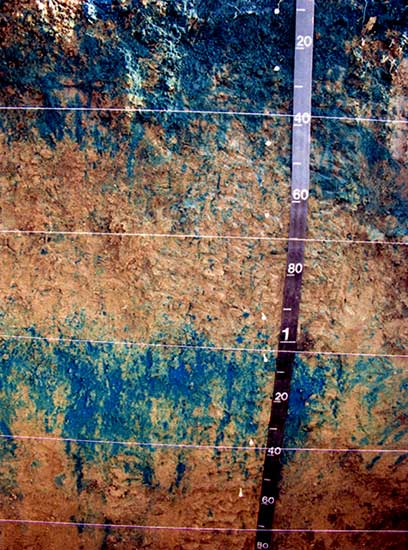
Figure 14--Site R8 Brilliant Blue dye pattern detail showing that the dye, being under tension, bypasses coarser textured soil.
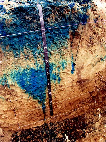
For site N7 in Ulysses soil, the dye pattern was different, forming a giant funnel front ending in a big finger down to approximately 6.6 ft, as shown in figure 15. Closer examination of a side finger, indicated in figure 16, showed that the dye finger formed along a decaying root channel, as did other fingers examined in both sites.
Figure 15--Funnel front pattern from Brilliant Blue dye tracer experiment at site N7.
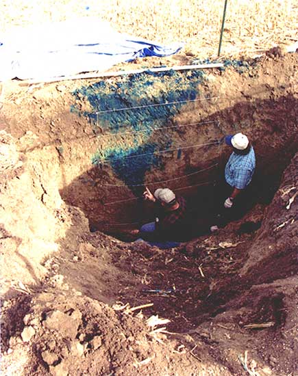
Figure 16--Closer up view of the funnel-front dye pattern and side finger formed along a decaying root channel.
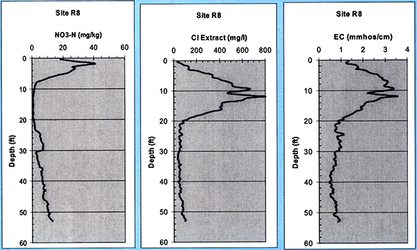
The nitrate, chloride, and electrical conductivity of collected soil cores were analyzed in 15.2-cm (6-in) increments down to 50 ft at the Servi-Tech Inc. laboratories in Dodge City, Kansas. For site R8 (with a long-term wastewater irrigation history-since 1986) we see (Fig. 17) a high nitrate peak of about 40 mg/kg around 2 ft, which decreases sharply in the depth interval of 10 to 20 ft, possibly due to alfalfa roots consuming the nitrate at those depths, as the R8 site was under alfalfa cultivation from 1997 to 2002. The nitrate picks up again reaching a secondary maximum near the depth of 30 ft, then following a decrease near that level, it progressively increases with depth down to more than 50 ft. It seems that a previous nitrate front has reached down to 30 ft, with yet older fronts making it down deeper, indicating that nitrate may had already penetrated down to those depths. The chloride and EC profiles show a peak around the depth of 10 to 12 ft, and follow a near-constant low profile below 20 ft.
Figure 17--Soil nitrate, chloride, and electrical conductivity (EC) profiles at site R8.
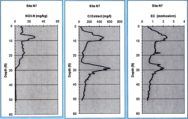
For site N7 (with wastewater irrigation history since 1998) we see (Fig. 18) a deeper nitrate peak (of less than 28 mg/kg, i.e., not as high as that at site R8) around 7 to 8 ft, which coincides with corresponding Chloride and EC peaks at that level. Then, the nitrate distribution progressively decreases to a minimal, background level by the time we reach to near 30 ft, indicating that nitrate penetrated down to near 30 ft but no further. A second chloride and EC peak occurs just above that 30-ft level.
Figure 18--Soil nitrate, chloride, and electrical conductivity (EC) profiles at site N7.
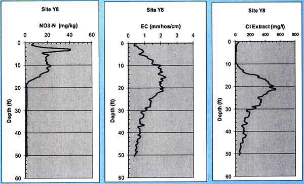
Finally, for site Y8 (without any wastewater irrigation), we see (Fig. 19) a high chloride peak around the 3-ft level, but by the time we reached the 18-ft depth level, nitrate goes back to minimal, background level. However, the Chloride and EC profiles reach a peak around that depth level. Site Y8 was planted with milo during 2005.
Figure 19--Soil nitrate, chloride, and electrical conductivity (EC) profiles at site Y8.
The sites were periodically irrigated from mid-May until the latter part of August 2005. The general quality of the treated wastewater effluent applied at the sites during 2005 is shown in figure 20. The chloride concentrations (in green) were around the 300 mg/L level, and the total Kjeldahl nitrogen concentrations (TKN, in blue) were around the 75 mg/L level.
Figure 20--Treated effluent irrigation water chloride, total Kjeldahl nitrogen, and nitrate-nitrogen concentration time series applied to sites R8 and N7 during 2005.
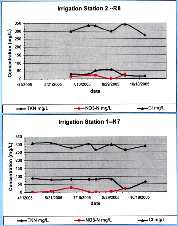
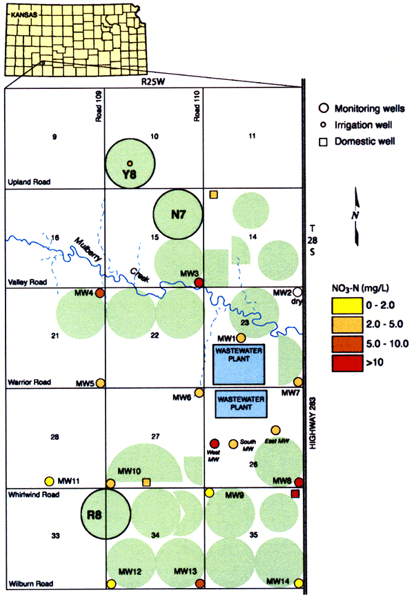
Figure 21 shows the groundwater nitrate-N concentrations from the November, 2005 survey sampling, where wells shown in red color exceed the safe drinking water limit for nitrateN of 10 mg/L. Notice that most of the wells have more than 2 mg/L nitrate-N in the groundwater. This indicates that anthropogenic sources have begun to impact the groundwater in the area. The 2 mg/L level is from work by the USGS on the National Water Quality Assessment program (Mueller and Helsel, 1996). Evaluation of the water chemistry in the appendices shows that the majority of the nitrogen in the lagoon wastewater used for irrigation is in the ammonium-N. The lysimeters show exceedingly high nitrate-N values and the monitoring and domestic wells have nitrate-N values generally above 2 mg/L. The change from the ammonium form in the wastewater to nitrate in the soil water is related to oxidation during the water treatment process and also to nitrification of the ammonium to nitrate by bacteria when the wastewater is applied. Nitrogen that is not utilized by the plants is available for leaching and moving to the groundwater.
Figure 21--Groundwater nitrate-nitrogen concentrations during November 2005.
Comparison of the nitrate-N values in lysimeter water samples (Tables 6 and 7) with soil core samples shows that although there is a large amount of nitrogen stored in the soil profile, an even larger amount is moving with the soil water that is available during certain time periods most likely related to rainfall and irrigation events. Chemically the lysimeter samples show higher concentrations of constituents (such as chloride or indicated by specific conductance values, Tables 6 and 7) than either the wastewater used for irrigation or the sampled ground water (Appendices B-D). Most likely this is related to evapoconcentration of applied constituents during the growing season and possible dissolution of stored salts in the soil profile. The EC and chloride profiles in the soils indicate that high salt profiles exist throughout the unsaturated zone and this is reflected in the shallow and medium lysimeter chemistries (Tables 6 and 7).
Table 6--Site R8 comparison of soil core and lysimeter samples for nitrate-N chloride and specific conductance (SPCD). Core nitrate-N samples converted from mg/kg using bulk density and moisture measurements.
| Site R8 | Depth (ft) |
Nitrate-N (mg/L) |
Chloride (mg/L) |
SPCD µS/cm |
|---|---|---|---|---|
| Lysimeter | 5.5 | 148.0 | 793 | 6030 |
| Soil Core | 5.5 | 72.8 | 336 | 2740 |
| L simeter | 26.5 | 55.9 | 250 | 2970 |
| Soil Core | 26.5 | 24.2 | 61 | 980 |
Table 7--Site N7 comparison of soil core and lysimeter samples for nitrate-N chloride and specific conductance (SPCD). Core nitrate-N samples converted from mg/kg using bulk density and moisture measurements.
| Site N7 | Depth (ft) |
Nitrate-N (mg/L) |
Chloride (mg/L) |
SPCD µS/cm |
|---|---|---|---|---|
| Soil Core | 17 | 54.7 | 85 | 1240 |
| Soil Core | 18 | 60.8 | 82 | 1270 |
| Lysimeter | 17.5 | 117 | 376.7 | 3142 |
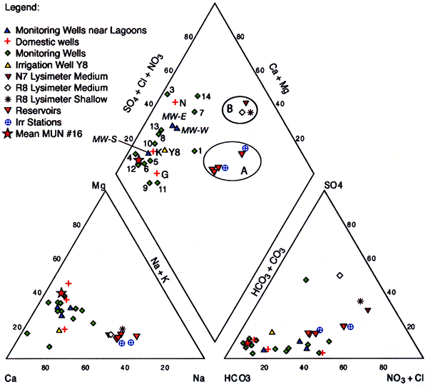
Water can be classified based on the quantity of dissolved constituents present in solution. The wastewater used for irrigation is classified generally a sodium-calcium-bicarbonate-nitrate-chloride water as compared to the water at Y8 which is a calcium-bicarbonate water (Fig. 22). The water type for the lysimeters are generally sodium-calcium-nitrate-chloride-sulfate waters. The variations in the "water-types" is indicative of the different water sources and processing that has affected the chemistry of the water. Analyses for the monitoring, domestic, and irrigation wells sampled during the study as well as for the wastewater and lysimeter samples are presented in Appendices B-D.
Figure 22 displays a trilinear diagram showing the average water quality of the irrigation water applied in both R8 and N7 sites marked as the A circle, the shallow and intermediate-depth suction lysimeter-sampled pore water from both sites marked as the B circle, and all sampled domestic, monitoring, and irrigation wells in the area left unmarked. All three sampled populations of applied wastewater, pore water from suction lysimeters, and monitoring and domestic wells form distinct groups in the trilinear diagram. The Dodge City municipal water sample from well #16 is also shown for comparison. This sample is the average of samples collected from 1990-2000 by the Kansas Department of Health and Environment (KDHE) for their annual water quality survey. The sample falls in the range of the low nitrate-N, low chloride monitoring well samples that have not been impacted by wastewater irrigation at this time.
Figure 22--Trilinear diagram showing the average 2005 water quality of irrigation water applied in sites R8 and N7 (circle A), the shallow and intermediate-depth suction lysimeter-sampled pore water from sites R8 and N7 (circle B), and all sampled domestic, monitoring, and irrigation wells in the area. Included in the graph is the mean city water analysis (star) for well #16 which was used in the annual water quality survey conducted by KDHE (1990-2000).
The ground-water samples, wastewater reservoirs, and lysimeter water are statistically different based on the Kruskal-Wallis non-parametric test for group differences of nitrate-N and conductivity (Tables 8 and 9). Samples were divided into groups based on water source. The Kruskal-Wallis test is a hypothesis test that at least one of the groups is different from the others. Examination of the statistical results indicates that the groups are different for both the nitrate-N and specific conductance values.
Table 8--Kruskal-Wallis test of nitrate-N differences based on water-source within the study area.
| Nitrate-N by water source (mg/L) |
Number of Samples |
Median Value Nitrate-N |
Kruskal-Wallis p value |
|---|---|---|---|
| Reservoir | 6 | 3.15 | 2.79 x 10⁻⁷ |
| Groundwater | 21 | 3.5 | |
| Lysimeters | 3 | 117.0 |
Table 9--Kruskal-Wallis test of specific conductance (SPCD) differences based on water-source within the study area.
| SPCD µS/cm by well type |
Number of Samples |
Median Value SPCD |
Kruskal- Wallis p value |
|---|---|---|---|
| Reservoir | 6 | 2334 | 1.43 x 10⁻⁷ |
| Groundwater | 21 | 484 | |
| Lysimeters | 3 | 3142 |
Site R8 has been under treated wastewater irrigation since 1996, site N7 since 1998, and site Y8 was never irrigated with treated wastewater. The land use/cropping practices at the field sites were clarified by the farmer Mr. Chuck Nickolson who manages the farms. Sites R8 and N7 were planted in corn on April 22 and 23,2005 and harvested in September 28 and 29, 2005, whereas site Y8 was planted in milo. The farmer planted 32,500 seeds of corn per acre in sites R8 and N7 in 30-inch ridge centers.
The land use practices followed at the sites are as follows: On the first week of April, 2005 the sites were sprayed with herbicides Roundup and 2-4D for weed control. A second spraying took place two weeks later. During the third week of June, 2005 the farmer created ridges in the field of approximately 6-inch height using appropriate tractor equipment. On the third and fourth week in June, 2005 the farmer applied 1.5 pounds active ingredient of the herbicide Atrazine per acre. Following harvesting, the farmer did stock chopping in November and December.
The LEPA irrigation sprinkler system (with drop nozzles) makes 2.5 circles per week to irrigate, and applies 0.75 inches of water per circle. The center pivots are equipped with water meters. The schedule of irrigation at the sites was obtained from Mr. Nickolson and the water meter was read each time neutron probe soil profile readings were made. He noted that the sprinkler irrigation system was running non-stop from July 21 to August 22, 2005 for both sites, except that it was shut off on August 2nd and restarted on August 300,2005.
The history of cultivation of sites R8 and N7 is as follows: Site R8 was planted in corn from 2003 to the present. From 1997 to 2002 it was planted in alfalfa. From 1996 to 1997 it was planted in wheat, and in 1996 it was planted in com. In contrast, site N7 was planted in corn from 1998 to the present. Prior to 1998, N7 was under a dryland wheat-fallow-wheat rotation.
All the information we collected from core analyses, neutron probe readings, dye tracer experiments, plus meteorologic information, and information on crop, irrigation, and other land use practices, is now being used in the RZWQM model to evaluate the environmental impacts of this treated wastewater irrigation process.
Sophocleous, Marios, Townsend, Margaret, A., 2006. Fate of nitrate beneath fields irrigated with treated wastewater, Ford County, KS: Hydrogeology-In-Progress seminar, Department of Geology, University of Kansas, Lawrence, KS, March 8, 2006.
Sophocleous, Marios, Townsend, M.A., Willson, T., Vocasek, F., 2006. Fate of nitrate beneath fields irrigated with treated wastewater, Ford County, KS: 2300 Annual Water and the Future of Kansas Conference, Oral Abstracts, Topeka, KS, March 16,2006.
Sophocleous, Marios, 2006. Preferential flow and transport of nitrate beneath treated wastewater-irrigated fields: Kansas Geological Survey Advisory Council, Lawrence, KS, March 31, 2006.
See Publications and Presentations above. In addition, Dodge City TV broadcasting news services recorded our dye-tracer experiments in November 2005 and interviewed co-PI Fred Vocasek on this project. See also Student Support below.
A graduate student in the School of Engineering of the University of Kansas is being supported by this project. Main duties include data processing and numerical modeling. An additional hourly student from Kansas State University based in the Garden City Agricultural Experiment Station is being supported for conducting periodic neutron moisture content readings at the field sites.
Numerous people and agencies assisted us during the conduct of this study, and they are listed below as a token of our gratitude.
KWRI: Funding source
NRCS: J. Warner, S. Graber, R. Still, T. Cochran, and C. Watts Servi-Tech: David Shuette
KSU-Extension: Fay Russett
OMI (Dodge City): Peggy Pearman, and Cliff Mastin Farm operator: Chuck Nicholson
Geoprobe Systems: Wes McCall
KGS: J. Healey, B. Engard, D. Thiele, R. Ghijsen, and J. Charlton
Graduate students: VinayKumar Muralidharan (KGS current), Qinghua Zhang (KGS previous), and Amanda Feldt (KSU-Extension)
Ahuja, L.R., DeCoursey, D.G., Barnes, B.B., and Rojas, K.W., 1993, Characteristics of macropore transport studied with the ARS Root Zone Water Quality Model: Transactions of the ASAE, vol. 36, no. 2, p. 369-380.
Ahuja, L.R., Rojas, K.W., Hanson, J.D., Shaffer, M. J., and Ma, L. (eds.), 2000, Root Zone Water Quality Model. Modeling management effects on water quality and crop production: Water Resources Publications, LLC, Highlands Ranch, CO, 372 p.
Asano, T., 1989, Irrigation with reclaimed municipal wastewater: California experiences; in Reuse of low quality water for irrigation, Bari, R. Bouchet, editor: CIHEAM, 1989, p. 119-132 (Options Méditerranéennes : Série A. Séminaires Méditerranéens; n. 1) [available online]
Avnimelech, Y., 1993, Irrigation with sewage effluents: the Israeli experience: Environmental Science and Technology, v. 27, no. 7, p. 1278-1280.
Ayers, R.S. and Westcot, D.W., 1989, Water Quality for Agriculture: FAO Irrigation and Drainage Paper, 29 Rev. 1. [available online]
Babcock, M., Picchioni, G.A, Mexal, J. G., and Ruiz, A., 2005, Land application of industrial wastewater on a Chihuahuan desert ecosystem: Fourth Annual Rio Grande Basin Initiatives Conference, Alpine, TX, April 12-14, 2005, poster. [PDF Online]
Bouma, J., Jongerius, A., Boersma, O., Jager, A, and Schoonderbeek, D., 1977, The function of different types of macropores during saturated flow through four swelling soil horizons: Soil Sci. Soc. Am. Jour., 41: 945-950.
Bouma, J. and van Lanen, J.A.J., 1987, Transfer functions and threshold values: From soil characteristics to land qualities; in Quantified land evaluation, K.J. Beek et al., editor: International Institute Aerospace Survey Earth Sci., ITC publ. 6. Enschede, the Netherlands, p. 106-110.
Bouwer, H., 1992, Agricultural and municipal use of wastewater: Water Science and Technology, vol. 26, no. 7-8, p. 1583-1591.
Brooks, R.H., and Corey, A.T., 1964, Hydraulic properties of porous media: Hydrology Paper 3, Colorado State Univ., Fort Collins, CO. [available online]
Dodge, D. A, Tomasu, B. I., Haberman, R. L., Roth, W. E., and Baumann, J. B., 1965. Soil Survey Ford County, Kansas: USDA Soil Conservation Service, Series 1958, no. 32, 84 p.
Flury M., Fluhler, H., Jury, W. A, and Leuenberger, J., 1994a, Susceptibility of soils to preferential flow of water: A field study: Water Resources Research, vol. 30, no. 7, p. 1945-1954.
Flury, M., and Fluhler, H., 1994b, Brilliant blue FCF as a dye tracer for solute transport studies--A toxicological overview: Environ. Qual. vol. 23, no. p. 1108-1112.
Flury, M. and Fluhler, H., 1995, Tracer characteristics of brilliant blue FCF: Soil Sci. Soc. Am. Journal, v. 59, p. 22-27.
Flury, Markus, and Wai, Nu Nu, 2003, Dyes as tracers for vadose zone hydrology: Reviews of Geophysics, vol. 41, issue 1, 1002. [available online]
Hathaway, L. R., Magnuson, L. M., Carr, B. L., Galle, O. K., and Waugh, T. C., 1975. Chemical quality of irrigation waters in west-central Kansas: Kansas Geological Survey, Chemical Quality Series 2, 46 p. [available online]
Hathaway, L. R., 1990, Nitrate UV-spectrophotometric screening method for the Technicon Autoanalyzer II System: Kansas Geological Survey, Open-file Report no. 90-49, 4 p.
Hayes, G. J. and DeWalle, Foppe, 1993, Irrigating with municipal sewage effluent in a rural environment: Journal of Environmental Science and Health, vo. A28, no. 6, p. 1229-1247.
Hogg, T.J., Weiterman, G., and Tollefson, L.C., 2003, Effluent Irrigation: Saskatchewan Perspective. [available online]
Jarvis, N.J., Hollis, J.M., Nicholls, P.H., Mayr, T., and Evans, S.P., 1997, MACRO-DB: a decision-support tool for assessing pesticide fate and mobility in soils: Environmental Modeling & Software, 12(2-3): 251-265.
Klute, A., ed. 1986, Methods of soil analysis, Part 1: Physical and mineralogical methods, second Edition. Monogr. 9. ASA and SSA, Madison, WI.
Larsson, M.H., and Jarvis, N.J., 1999, Evaluation of a dual porosity model to predict field-scale solute transport in a macroporous soil: Jour. Hydrology, 215: 153-171.
Logsdon, S.D., 2002, Determination of preferential flow model parameters: Soil Sci. Soc. Am. Jour., 66: 1095-1103.
Millard, S. P., 2002, Environmental Stats for S-PLUS, hypothesis test for k samples, Levene's Test for homogeneity of variance: Version 2.0. Release 1 for Microsoft Windows.
Mualem, Y., 1976, A new model predicting the hydraulic conductivity of unsaturated porous media. Water Resour., Res. vol. 12, p. 513-522.
Mueller, D. K. and Helsel, D. R., 1996, Nutrients in the nation's waters too much of a good thing?: U. S. Geological Survey, Circular 1136, 24 p. [available online]
Nemes, A., Schaap, M.G., and Wosten, J.H.M., 2003, Functional evaluation of pedotransfer functions derived from different scales of data collection: Soil Sci. Soc. Am. Jour., vol. 67, p. 1093-1102.
Petersen, C. T., Hansen, S., and Jensen, H. E., 1997, Depth distribution of preferential flow patterns in a sandy loam soil as affected by tillage: Hydrology and Earth System Sciences, vol. 4, p. 769-776.
Rawls, W. J., Ahuja, L. R., and Brakensiek, D. L., 1992, Estimating soil hydraulic properties from soils data; in, Indirect methods for estimating the hydraulic properties of unsaturated soils, M. Th. Van Genuchten, F. J. Leij, and L.J. Lund, editors: Proc. Int Worksh. Riverside, CA. Oct 11-13, 1989. University of California, Riverside, CA, p. 329-340.
Rawls, W.J., Brakensiek, D.L., and Logsdon, S.D., 1996, Estimation of macro pore properties for no-till soils: Transactions of the ASAE, 39(1): 91-95.
Schaap, M.G. and Bouten, W., 1996, Modeling water retention curves of sandy soils using neural networks: Water Resour. Res. 32:3033-3040.
Schaap, M.G., Leij, F. J., and van Genuchten, M. Th., 1998a, Neural network analysis for hierarchical prediction of soil water retention and saturated hydraulic conductivity: Soil Sci. Soc. Am. J. 62:847-855.
Schaap, M.G., and Leij, F.J., 1998a, Using Neural Networks to predict soil water retention and soil hydraulic conductivity: Soil & Tillage Research 47:37-42.
Schaap, M.G., and Leij, F.J., 1998b, Database Related Accuracy and Uncertainty of Pedotransfer Functions: Soil Science 163:765-779.
Vacasek, F., 2006, Soil and effluent monitoring, Annual Report: Year Nineteen (2005): Report (Project Number: 05-001c) submitted to Operations Management International, Dodge City, KS, Servi-Tech, Inc., Dodge City, KS, 23 p. plus Tables and Figures.
Wosten, J.H.M., Pachepsky, Ya. A., and Rawls, W.J., 2001. Pedotransfer functions: bridging the gap between available basic soil data and missing soil hydraulics characteristics: Jour. Hydrology, 251: 123-150.
Zupancic, J. W. and Vocasek, F. F., 2002, Dealing with changes in volume and quality of effluent at the Dodge City wastewater recycling project over the last sixteen years--1986 through 2001: 2002 Technical Conference Proceedings of the Irrigation Association, New Orleans, Louisiana.
Kansas Geological Survey, Geohydrology
Placed online July 29, 2014
Comments to webadmin@kgs.ku.edu
The URL for this page is http://www.kgs.ku.edu/Hydro/Publications/2007/OFR07_14/index.html