Kansas Geological Survey, Open-file Report 2004-46
by
Marios Sophocleous1, Earl Bardsley2, John Healey1, and Brett Engard1
1Kansas Geological Survey, The University of Kansas, Lawrence, KS 66047, USA
2Department of Earth Sciences, University of Waikato, Hamilton, New Zealand
KGS Open File Report 2004-46
October 2004
Most multi-year water-level records exhibit regular annual fluctuations. For shallow wells, these fluctuations are clearly caused by seasonal recharge to the aquifers in which the wells are completed. However, groundwater levels may change as a result of natural causes other than recharge. In particular, it is well known that loading effects such as those owing to changes in barometric pressures or ocean tides will result in groundwater-level fluctuations, even in deep confined aquifers (e.g. Jacob, 1940). These fluctuations are the consequence of changes in mechanical loads (stresses) at the ground surface that are transmitted instantaneously to underlying formations and need not involve any flow. The resulting changes of total stress are evidenced by corresponding changes of pore pressure. In thick, low-permeability formations fast drainage does not happen and the pore-pressure transients are exactly proportional to changes of surface load.
The response of groundwater pressure to changes of barometric pressure, observed in most water wells, is a familiar example of this effect (e.g. Freeze and Cherry, 1979). An increase of water loading may also arise from rainwater accumulating in the soil profile or water table. The result (in the absence of other effects) is a progressive increase in pore-water pressure in the confined aquifer. Conversely, decreases in water loading will occur whenever near-surface water mass is reduced by evaporation or net lateral groundwater export. These loading effects are independent of changes associated with recharge to the confined aquifer.
Earlier research of van der Kamp and Maathuis (1991) in Canada and Bardsley and Campbell (1994) in New Zealand showed that seasonal changes of groundwater pressure in highly permeable, deep aquifers are related to seasonal surface-loading effects. Such responses of confined aquifers to changes of overlying loading effects can be thought of as "piezometric weighing lysimeters" (van der Kamp and Maathuis, 1991) or "geologic weighing lysimeters" (Bardsley and Campbell, 2000), that is, natural, giant weighing lysimeters that track changes of total water balance over an area of tens of hectares. Highly accurate monitoring of changes in groundwater pressure in groundwater environments where deep recharge is minimal offers a unique opportunity to obtain hydrologic data at a scale that is much larger than that of "point" measurements, but smaller than whole-watershed observations such as streamflow.
It is helpful to make a distinction between barometric and loading effects as factors influencing a water-level time series obtained from a well emplaced in a confined formation (Bardsley and Campbell, 2000). Given that the well is exposed to the atmosphere, the well barometric effect causes the well water level to fall as atmospheric pressure increases, and vice versa. In contrast, a mass load added to the land surface causes the well water level to rise, and a removal of mass causes the level to fall.
The amount of well water-level change caused by a loading change is quantified by the "loading coefficent", c, where c = 1 - b (Jacob, 1940), and b is the "barometric efficiency," which is a proportionality constant that quantifies the extent to which the formation pore-water pressure near the well "feels" changes in atmospheric pressure.
Water loading tends to be cumulative and hence may have a significant effect on seasonal time scales (Bardsley and Campbell, 1995). For example, the water accumulated from individual winter rainfalls may cause a loading increase of magnitude and duration greater than any barometric effect. For example, recall that the change of piezometric head in response to water loading is given by (1-b) L, where L is the depth-equivalent of accumulated near-surface water and b is the barometric efficiency of the confined aquifer. A barometric efficiency of 0.2 combined with 50 cm of accumulated water would create a 40-cm rise in confined-aquifer piezometric level.
Seasonal variation of water-table levels represents an obvious indication of changes in near-surface water loading. As Bardsley and Campbell (1995) also pointed out, it is surprising then that there has been no prior recognition that these loading changes imply synchronous seasonal variation of piezometric head in any deeper confined aquifer. At least one major groundwater text even excludes the possibility of seasonal external loading (Freeze and Cherry, 1979, p. 230).
Water loading possibly has gone unrecognized for so long because piezometric-data sequences often have time resolutions no better than a day, while hourly recordings of confined-aquifer piezometric levels are needed to show the near-instantaneous loading increments associated with individual rainfall events (Bardsley and Campbell, 1994).
The spatial extent of the system's response can be estimated from the theory for point loads (van der Kamp et al., 2003). Roughly speaking, 90% of the pore pressure response is due to surface loading within a radius equal to 10 times the depth of the piezometer intake (van der Kamp and Schmidt, 1997). Thus a 30-m-deep installation will reflect hydrologic changes over an area of tens of hectares. Ideally, therefore, the lysimeters should be installed within hydrologically uniform areas that extend for at least several hundred meters in all directions.
Thus, deeper formations will "weigh" surface water budget changes over larger land areas. The deepest formation in the New Zealand experiment (Bardsley and Campbell, 1994, 2000) was 160 m below ground surface. Bardsley and Campbell (2000) noted apparent geological weighing behavior in a formation 240 m below ground surface as part of an earthquake field study near Parkfield, California. Presumably some depth limit exists, beyond which deep formations no longer detect surface loading changes; however, such a limit has not yet been established. A detailed earth-loading model suggests that surface load deformation should penetrate to a depth about twice the lateral extent of the load (Pagiatakis, 1990).
The purpose of this note is to demonstrate that we have detected such rainfall loading effects in a nearly 300-m-deep Upper Dakota Formation observation well near WaKeeney, west-central Kansas, and that this observation, to our knowledge, represents the clearest signal of rainfall loading at depth to date.
The site of the WaKeeney monitoring well is in Trego County in western Kansas, approximately 7.6 km northwest of the town of WaKeeney (Fig. 1; Hodson, 1965). The area lies within the High Plains physiographic province of western Kansas and is characterized by gently rolling uplands that are moderately dissected by smaller drainageways.
Figure 1. Location of the WaKeeney well site and area geology (Modified from Hodson, 1965).
The area has a semiarid continental climate characterized by low to moderate precipitation [the mean annual precipitation at WaKeeney is 544 mm based on the period 1931-1955 (Hodson, 1965) or 594 mm based on the period 1951-1976 (Watts et al., 1990)], a high rate of evaporation [total annual reference (potential) evapotranspiration for the year 2003 (based on the Hill City station in the neighboring county to the north) was 1913 mm], reasonably mild winters with relatively little snowfall, and fairly hot summers [in winter, the average temperature is -0.44 °C and in summer, the average temperature is 24.2 °C (Watts et al., 1990)]. Approximately 70% of the annual precipitation in Trego County falls during the growing season of April through September.
The rocks that crop out in the area are sedimentary in origin and range in age from Cretaceous to Holocene. Their areal distribution is shown in Fig. 1. A drilled section of the rock units at the site is given in Fig. 2. Alluvium of late Wisconsinan and Holocene age occurs along the principal streams and smaller valleys in the county and constitutes an important source of groundwater in Trego County. The Pleistocene Series is represented by unconsolidated deposits of both fluviatile and eolian origin that generally yield small to adequate water supplies for domestic and stock supplies. Thin eolian silts (loess) of late Pleistocene age cover a considerable part of Trego County and are shown as the Peoria and Loveland Formations undifferentiated in Fig. 1. The Ogallala Formation of Pliocene age unconformably overlies the Cretaceous rocks in much of the upland areas of the county and consists predominantly of sand, gravel, silt, and clay. The Ogallala Formation is the most widespread shallow water-bearing formation in Trego County, although its thickness is relatively small compared to further west.
Figure 2. Subsurface stratigraphy and well construction of the WaKeeney well.
The Niobrara Chalk of Late Cretaceous age crops out along the river valleys and their tributaries and consists chiefly of alternating beds of light-gray chalk, chalky limestone, and chalky shale (Hodson, 1965). The beds of shaly chalk are relatively impermeable and water is transmitted chiefly through joints and fractures only locally and in small quantities. The Niobrara Chalk is divided into two members, the Fort Hays Limestone below and the Smoky Hill Chalk above. The Carlile shale of Late Cretaceous age consists of the Fairport Chalk Member (lowermost), the Blue Hill Shale Member, and the Codell Sandstone Member (uppermost), which locally yields small amounts of water to wells. The Greenhorn Limestone consists principally of alternating thin beds of chalky limestone and marl, which are both relatively impervious and do not yield water to wells. Underlying the Greenhorn Limestone is the Graneros Shale, which consists chiefly of dark-gray to black noncalcareous shale and yields no water to wells (Hodson, 1965).
Finally, the Dakota Formation of Early Cretaceous age consists chiefly of varicolored clay containing irregular, lenticular beds of siltstone and sandstone and yields quantities of water sufficient only for domestic or stock supplies. The depth to the Dakota Formation at the WaKeeney site is approximately 235 m (770 ft) or greater below ground surface, whereas the depth to the water level at the site is approximately 132.4 m (434.5 ft) below ground surface. Obviously the sandstone lenses of the Dakota Formation are under significant confining pressure, being confined by hundreds of feet of relatively impervious shaly and chalky formations and adjacent Dakota siltstones. As a result, any downward recharge through the thick confining layers to the deep Dakota aquifer seems unlikely at the site.
Figure 2 also shows the WaKeeney well-construction details and other relevant information. Hourly measurements of water levels have been recorded since early January 2004 using a minitroll pressure transducer. Hourly barometric-pressure data are available for the Hill City weather station some 30 km north of the site, whereas daily precipitation data are available from a weather station in the nearby town of WaKeeney as well as from a USGS stream-gaging station of the Saline River near WaKeeney (Fig. 1) equipped with a tipping-bucket raingage approximately 8 km northeast of the site.
The ratio of the change in the water level in a well to the change in atmospheric pressure that produces it is known as barometric efficiency. Fluctuations of the water level caused by changes in atmospheric pressure (as shown in Fig. 3 from our Dakota observation well near WaKeeney, Kansas) often obscure other fluctuations that are of interest in hydrologic studies. Evaluating and eliminating the atmospheric fluctuations from the water-level record is therefore necessary. To do this, the barometric efficiency of the well must be determined.
Figure 3. Fluctuations of area barometric pressure and water level at the WaKeeney well. A larger version of this figure is available.
The barometric efficiency of a well is usually determined by a number of methods. In our case we used the following three methods: (1) by plotting the water-level changes as ordinates and the corresponding changes in barometric pressure on rectangular paper, both expressed as a column of water. The slope of the straight line drawn through the plotted points is the barometric efficiency; (2) by plotting water levels in the y-axis against atmospheric pressure (expressed as a column of water) on the x-axis, the slope of the straight line being the barometric efficiency (Brassington, 1998); and (3) by plotting a summation plot of the incremental changes in water level versus the incremental change in atmospheric pressure following appropriate summation rules specified by Clark (1967).
A barometric efficiency of 1.0 indicates that 1 cm of change in barometric pressure (in equivalent cm of water) results in 1 cm of change in water level, whereas a barometric efficiency of 0.0 indicates that barometric-pressure changes have no effect on water levels. High barometric efficiencies reflect high strength and rigid test formations, whereas low barometric efficiencies indicate highly compressive formations (Spane, 1999).
Using at least 2 months of hourly water-level and barometric-pressure data, the WaKeeney well barometric-efficiency estimates using each one of the above-mentioned techniques are shown in Table 1.
Table 1. Barometric efficiency estimates for the WaKeeney well
| Method | Estimate | Coefficient of determination, R2 |
|---|---|---|
| (1) Water-level/barom.-press. fluctuations | 0.627 | 0.534 |
| (2) Brassington's method | 0.631 | 0.951 |
| (3) Clark's method | 0.568 | 0.999 |
The results from Table 1 indicate a relatively high barometric efficiency for the WaKeeney well. Owing to the inverse relationship between barometric efficiency and loading efficiency (Jacob, 1940), a formation with a relatively high barometric efficiency would have a relatively low sensitivity to surface water loading effects, and this seems to be the case here. A relatively high barometric efficiency also leads to relatively high earth tide effects, which means that rainfall events have to be fairly big to register over the earth tide amplitudes.
If a given confined aquifer shows a barometrically corrected pore pressure change, ΔP, over some given time period. Δt, then this can be converted into an estimate of the area-integrated water-storage change, ΔS, by the relation
| ΔS=ΔP/(1-b) | (1) |
where b is the aquifer barometric coefficient and ΔS and ΔP are both expressed as water-length equivalents. Evaluating ΔS for a progressively incremented Δt gives the storage change as a function of time from arbitrary initial zero. Establishing the barometric coefficient of the geological units concerned allows the pore-water pressures to be corrected for atmospheric-pressure changes, with the rescaled residual being the estimated water-budget storage change. Correcting for mass increment gains due to precipitation events gives the local "water export function" (Bardsley and Campbell, 2000), which is the rate of local water loss from or near the ground surface due to the combined effects of evaporation, stream discharge, and any net lateral groundwater outflow.
The relation (1) is based on a number of assumptions. In particular, the aquifer is assumed to have pure vertical elastic response to changes in vertical stress, there are no dynamic sources of pore-water-pressure variation in the confined aquifer from recharge effects or water abstractions, and the aquifer concerned is fully confined with no hydraulic linkage to the confining units above and below. These assumptions, although difficult to confirm by direct means, are most probably true at the WaKeeney well site (see further below).
Although no significant precipitation events were recorded at the WaKeeney site during the October 2003 to May 2004 observation period (this field trial was established in October 2003--the area being in the midst of a major regional drought; the total precipitation from October 2003 to March 2004 being 33 mm, 38 mm for April 2004, and 22 mm for May 2004), the water-level observations at the WaKeeney well are consistent with a geological weighing lysimeter measuring total evaporation loss as shown in the "water-export curve" (Fig. 4). That curve was derived from subtracting cumulative rainfall from the aquifer-storage time series (based on eq. 1), thus resulting in the site water mass changes estimated from pore-water pressure measurements at 293-m depth excluding rainfall inputs, and shows that most of the annual precipitation input is exported as spring time advances via evaporation and shallow, unconfined aquifer net-lateral outflow, the clayey and confining nature of the sediments precluding much lateral deep groundwater import. Over the winter no water export is noted (Fig. 4), consistent with that season's minimal evaporation loss.
Figure 4. WaKeeney water-export trend, calculated by subtracting cumulative rainfall from the aquifer-storage change time series during the monitored period from October 3, 2003, to May 7, 2004. High frequency variations are due to earth-tide effects. A larger version of this figure is available.
The relatively high barometric efficiency of the Dakota aquifer at the WaKeeney site results in significant earth-tide amplitudes, which obscure the visibility of the individual relatively small precipitation-loading effects associated with the drought over the observation period. Given the relatively high barometric efficiency of the WaKeeney well and the persisting drought conditions resulting in minimal rainfall events too small to be distinguished from earth-tide amplitudes, how do we establish proof of the concept that surface loading (and by implication surface unloading) can be detected at depth? An indirect method of checking for loading effects can be achieved by regression analysis of the measured groundwater-level time series (yt) as a function of barometric pressure (Pt), cumulative precipitation (Rt), and time trend t, where the latter is approximated as a quadratic expression. This gives
| yt= b Pt + c Rt+ dt + constant | (2) |
where b, c, and d are regression coefficients (Bardsley and Campbell, 1994).
The geological weighing lysimeter theory predicts that b + c = 1.0 according to the standard theoretical model of Jacob (1940). We tested for loading effects in the WaKeeney data by estimating b, c, and d as independent regression parameters. All regression parameters in eq. (2) were significant, and in particular b = 0.621, and c = 0.385 which gives a sum to 1.006 ± 0.025, very close to the theoretical value of 1.0. All the parameter estimates collectively cause eq. (2) to yield a good fit (with Multiple R = 98.30% and Adjusted R2 = 96.62%).
In addition to the aforementioned statistical proof of concept, to further demonstrate loading effects under such circumstances (a combination of drought conditions and high barometric-efficiency formation), we took advantage of the loading impacts of the atmosphere itself by sealing off the top of the well with a suitable airtight seal so that atmospheric-pressure changes no longer had any direct influence on the water level in the well. Any fluctuations in well-water levels can then only come from land-surface loading effects felt directly by the deep aquifer.
The WaKeeney well steel casing with a bolted heavy steel plate on top was sealed by employing a rubber gasket between the top of the steel casing and the bolted steel plate (Fig. 5) on June 23, 2004, and an available Solinst mini LT levelogger pressure transducer sensor (LT F15/M5 with a range of 4m and a resolution of 0.2 cm) was installed inside the borehole air column (via a steel cable) to a depth of 7.36 m below ground surface to minimize temperature-fluctuation effects. The levelogger was programmed to log the borehole air column at half-hourly intervals to serve as a barologger to confirm that barometric variations are not getting in through the cased borehole. Figure 6 displays the results of this experiment: indeed the well-water level is fluctuating in parallel to atmospheric pressure (Fig. 6a), demonstrating that atmospheric loading is being felt directly by the deep Dakota aquifer, whereas the air-column pressure shows a near-horizontal line (some drift is apparent in the levelogger) demonstrating no atmospheric fluctuations (Fig. 6b). In the open-well case, the water-level fluctuations derived from the atmospheric effect are mirror-opposites of the barometric fluctuations (Fig. 3), i.e. when the barometric pressure increases, the water level decreases. In the sealed-well case, the water-level fluctuations derived from the atmospheric effect now have the same sign as the atmospheric-pressure changes (Fig. 6a); in other words, the atmosphere acts like a surface load that comes and goes--just like rainfall and evaporation.
Figure 5. The WaKeeney well steel casing with a bolted steel plate. The rubber gasket below the top steel plate to hermetically seal the well is visible in the picture.
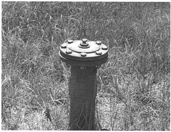
Figure 6. Results of the sealing experiment: (a) atmospheric pressure and water-level fluctuations; (b) wellbore air-column pressure and water-level fluctuations. A larger version of this figure is available.
At last, during the June 2004 time period following the sealing experiment (and during a few days prior to the June 22 start of the experiment, but not having the data available at the time) a number of big rainfall events (greater than 20 mm/day) occurred, with the largest one-day rainfall of more than 86 mm occurring in July 1, 2004. In addition, a series of consecutive rains during the period June 15 to June 21, 2004, dumped more than 90 mm over the area. Both the single July 1 and the combined June 15-21 rainfall events appear as clear step increments in the barometrically corrected water-level time series beyond the earth-tide range (Fig. 7). The combined June 15-21 rainfall total temporarily broke a midly declining water-level trend until the big rainfall event of July 1 added a nearly constant step increment to the corrected water-level time series until at least up to the end of the July 13, 2004, observation period (Fig. 7). The cumulative rainfall plot (Fig. 7) shows an almost exact coincidence in time with the rise in piezometer water, verifying that the aquifer gives an accurate proportional measure of the increased loading of the rainwater as it accumulates in the soil almost 300 m above! Of course, with a sealed well, the very fact that we were able to do a barometric correction is indicative of loading effects at a depth of approximately 300 m, with an ability to "weigh" an area of more than 2800 ha. The implication here is that deeper installations could "weigh" even larger areas.
Figure 7. Uncorrected (lighter line) and barometrically corrected (heavier line) water-level fluctuations and cumulative rainfall. The corrected water-level series from the upper Dakota Formation, almost 300 m below ground surface, displays earth-tide effects, and nearly instantly responds to surface-rainfall loading events. A larger version of this figure is available.
We would like to thank Mr. Larry Connor, the owner of the WaKeeney site for allowing us access to his property. Allen MacFarlane of the Kansas Geological Survey (KGS) for loaning us the minitroll datalogger used to measure the water levels reported here as well as his geophysical logging expertise. Jim Butler of the KGS also made available the levelogger used in the sealing experiment.
Bardsley, W.E., and Campbell, D.I., 1994. A new method for measuring near-surface moisture budgets in hydrological systems: Jour. Hydrology, 154(1-4): 245-254.
Bardsley, W.E., and Campbell, D.I. 1995. Water loading: a neglected factor in the analysis of piezometric time series from confined aquifers (Note). Jour. Hydrology (NZ), 34(2): 89-93.
Bardsley, W.E., and Campbell, D.I., 2000. Natural geological weighing lysimeters: calibration tools for satellite and ground surface gravity monitoring of subsurface water mass change. Natural Resources Research, 9(2): 147-156.
Brassington, R., 1998. Field Hydrogeology, 2nd ed., John Wiley & Sons, Chichester, England, 248 p.
Clark, W.E., 1967. Computing the barometric efficiency of a well: Am. Soc. Civil Engineers, Jour. Hydraulic Div., Proc., 93(HY 4): 93-98.
Freeze, R.A., and Cherry, J.A., 1979. Groundwater. Prentice-Hall, Englewood Cliffs, New Jersey.
Hodson, W.G., 1965. Geology and groundwater resources of Trego County, Kansas. Kansas Geol. Survey, Bull. 174, 80 p.
Jacob, C.E., 1940. On the flow of water in an artesian aquifer: Eos Trans. AGU., 21: 574-586.
Pagiatakis, S.D., 1990. The response of a realistic Earth to ocean tide loading: Geophysical Jour. Intern., 103(2): 541-560.
Spane, F.A., Jr., 1999. Effects of barometric fluctuations on well water-level measurements and aquifer test data: Pacific Northwest National Lab., PNNL-13078, Richland, Washington, 45 p.
van der Kamp, G., and Maathuis, H., 1991. Annual fluctuations of groundwater levels due to loading by surface moisture. Jour. of Hydrology, 127: 137-152.
van der Kamp, G., and Schmidt, R., 1997. Monitoring of total soil moisture on a scale of hectares using groundwater piezometers. Geoph. Res. Lett., 24(6): 719-722.
van der Kamp, G., Barr, A., Granger, R., and Schmidt, R., 2003. Use of deep piezometers in aquitards for continuous monitoring of hectare-scale soil moisture balance. Proc. 4th Joint Groundwater Specialty Conf., Intern. Assoc. of Hydrogeologists--Canadian National Chapter, and Canadian Geotech. Soc., Sept. 29-Oct. 1, 2003, Winnipeg MB, Canada.
Watts, C.E., Palmer, C.D., and Glaum, S.A., 1990. Soil survey of Trego County, Kansas. U.S. Dept. of Agric., Natural Resourc. Conserv. Service, 114 p. plus map sheets.
Kansas Geological Survey, Geohydrology
Placed online Jan. 9, 2006
Comments to webadmin@kgs.ku.edu
The URL for this page is http://www.kgs.ku.edu/Hydro/Publications/2004/OFR04_46/index.html