Kansas Geological Survey, Open-file Report 1999-20
by
C. D. McElwee and G. C. Bohling
Prepared for Presentation at
Spring AGU Meeting, Boston, MA
June 3, 1999
KGS Open-file Report 1999-20
In many parts of the US, ground-water levels are declining and state or local agencies are involved in managing the aquifer to achieve certain goals. These goals might involve stabilizing the water levels, planning the depletion period, or evaluating the effect of certain withdrawal activities. Ground-water models are often used to give guidance in managing an aquifer but invariably contain uncertainty in the input data. Typically, model input will include estimates or measurements of such things as hydraulic conductivity, storativity, bedrock elevation, recharge/discharge, and water levels. Water levels are often calculated as a function of the other input variables and may be used in an inverse scheme to refine the estimates of the input variables. However, it is possible to consider the heads as input and to calculate the recharge/discharge or net flux of water at any location as the output. In either case, the calculated output contains uncertainty which is propagated from the input variables. This paper examines that problem by two methods: Monte Carlo analysis and first order sensitivity analysis. The Monte Carlo analysis has the advantage of giving the exact answer as the number of realizations used approaches a large number. However, it may be computationally intensive. First order sensitivity analysis is easier to do computationally but is only approximately correct. It predicts that the uncertainty distribution of the output variable is a sum of the uncertainty distributions of the input variables weighted by the sensitivity coefficients. This paper will present some comparisons of the two methods for calculating the output uncertainty distribution and will indicate some conditions under which the simpler first order sensitivity analysis may be used.
We will consider a steady state model for 1-D flow, such as along a streamline. The basic equation is given by (Hermance, 1999)
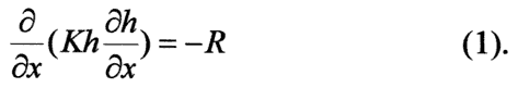
Where K is the hydraulic conductivity, h is the hydraulic head, and R is the net flux or recharge into or out of the model. We consider the case where K and R may vary over space.
Consider a discrete model with node point indices from 0 to N and constant node spacing of Δx (Wang and Anderson, 1982). The solution to equation (1) is
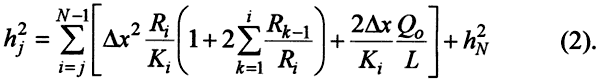
For an arbitrary distribution of K and R, the solution at node j is given by equation (2), where the boundary conditions are that the head is hN at node N and the flux per unit width is Q0/L at node zero. Equation (2) is a deterministic equation for head if K and R are known.
The problem that we want to investigate involves estimating the net flux or recharge (R) into the model at any node. In many ground water investigations head data have been measured in the field and hydraulic conductivity distributions can be estimated from drilling logs or geophysical methods. Invariably, these measurements will have error associated with them. We want to investigate how errors in the K and h data propagate into estimates for the recharge or net flux (R).
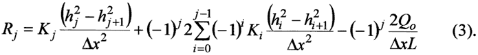
Equation (3) will estimate the recharge from any given K and h distribution. If there are errors in K and h these will be propagated into the estimates for R.
A second way to estimate the recharge is to take a numerical analog of equation (1).
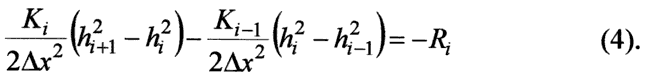
Equation (4) is much simpler to apply and is only based on conservation of water in a model cell.
A third estimator of the net flux or recharge can be obtained by realizing equation (1) implies that
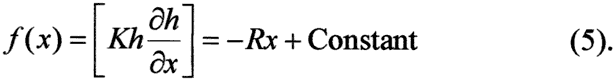
This means that if we calculate f(x) from the field data for K and h, it should fit a straight line for areas where R is constant. We can use a least squares method (Draper and Smith, 1998) to fit equation (5) to a given number of data points for f(x). This fitting procedure can be translated along the flow line to generate an estimate of R at each node point.
We used equation (2) to calculate exact head data for an assumed distribution for K and R. A standard Monte Carlo analysis (Benjamin and Cornell, 1970) was used to generate statistics for the recharge estimate methods. The exact head data and K distribution are corrupted with errors picked at random from Gaussian normal distributions with a given standard deviation to generate 1000 realizations of h and K. This data is then used in the above three methods for estimating R to generate 1000 realizations of the recharge distribution. Statistics are then collected on the 1000 R distributions to define the average value and standard deviation at each node point.
The error in recharge ΔR caused by changing the values of K and h by ΔK and Δh can be estimated with first order sensitivity analysis (McElwee, 1987).
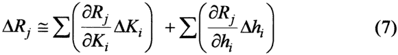
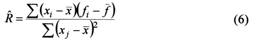
The partial derivatives of R with respect to K and h are called sensitivity coefficients. The standard deviation of the R distribution resulting from a Gaussian error distribution in K and h with standard deviations of σk and σh is given by (Benjamin and Cornell, 1970)
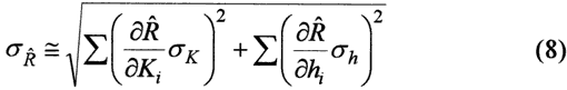
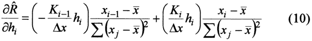
Equation (8) can be compared to the results of the Monte Carlo simulations. The sensitivity coefficients for the least squares fit of equation (6) are
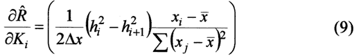
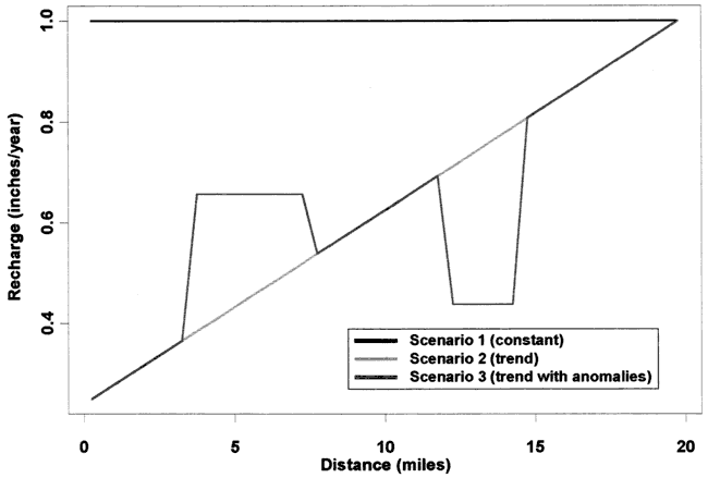
The three recharge scenarios that we consider are shown in Figure 1. We consider a 40 node model with one-half mile grid spacing and an average hydraulic conductivity of 50 ft/day. Scenario 1 considers constant recharge of 1 inch per year. Scenario 2 considers a linear trend of recharge increasing from 1/4 inch per year to 1 inch per year. Scenario 3 considers two anomalies in recharge superimposed on the linear trend. These numbers for hydraulic conductivity and recharge are similar to situations in the High Plains Aquifer of Kansas (Sophocleous, 1998).
Figure 1. Three recharge scenarios.
Hydraulic head profiles for these three recharge scenarios are shown in Figure 2. There is not much difference in the profiles for scenarios 2 and 3. In order to do Monte Carlo simulations for estimating the recharge, these head profiles are corrupted with Gaussian noise of zero mean and a certain standard deviation σh.
Figure 2. Head profiles for three recharge scenarios.
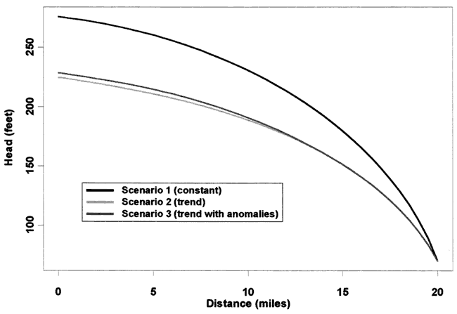
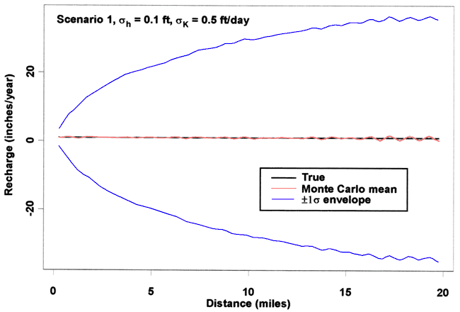
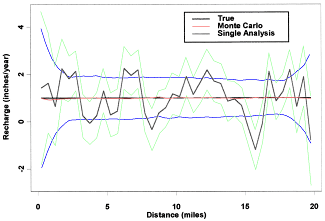
Figure 3 shows the results of applying method one to estimate the recharge in the presence of noise on h and K. A σk of 0.5 ft/day and a σh of 0.1 ft has been used. Figure 3 presents the Monte Carlo results for 1000 realizations of h and K profiles. Notice that even in the presence of this relatively small amount of noise, the error in recharge estimation grows along the flow direction and basically becomes unusable very quickly. This result is because the analytical solution for recharge given by equation (3) causes error to propagate as the calculation proceeds. It appears that this method is not feasible even with low levels of noise.
Figure 3. Recharge estimates from Method One.
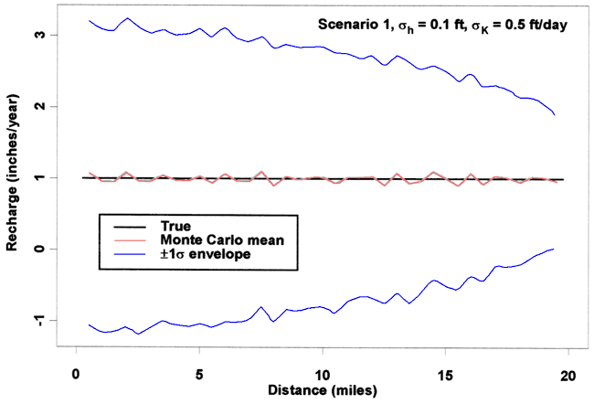
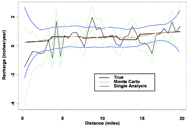
Method two results, using equation (4), are shown in Figure 4. Again, this figure presents Monte Carlo results for a σk of 0.5 ft/day and a σh of 0.1 ft. Although this method is better than method one, since the estimation error in R does not grow along the flowline, the error is still fairly large even for these relatively small magnitudes of noise.
Figure 4. Recharge estimates from Method Two.
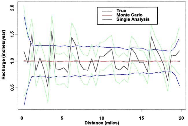
Method three attempts to smooth out some of the error by fitting a straight line to a number of points of the f(x) function [equation (5)] in order to estimate the recharge. This procedure is repeated for each node point by sliding the fitting window along the head profile. Monte Carlo calculations are used for 1000 realizations of the f(x) to collect statistics on R and its standard deviation. In addition, first order sensitivity analysis is used to estimate the one standard deviation bounds for one realization of R. Figure 5 shows the results for a σk of 0.5 ft/day and a σh of 0.1 ft and a fitting window including 5 points of f(x) for recharge scenario 1. The constant recharge value of 1 inch/yr is well represented by the Monte Carlo results and the one standard deviation lines indicate the recharge is being estimated to within about plus or minus 30%. On the other hand, the single realization of R plotted on Figure 5 is rather ragged. The first order sensitivity analysis estimate of the one standard deviation bounds on the single realization are essentially identical to the Monte Carlo results, although the center values are biased by the values of the single realization of R.
Figure 5. Scenario 1, σh of 0.1 ft, σk of 0.5 ft/day, 5-point fit.
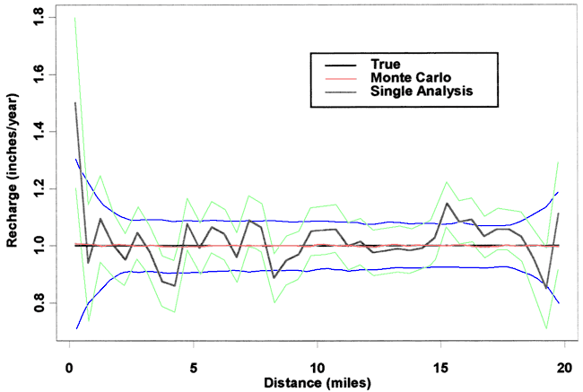
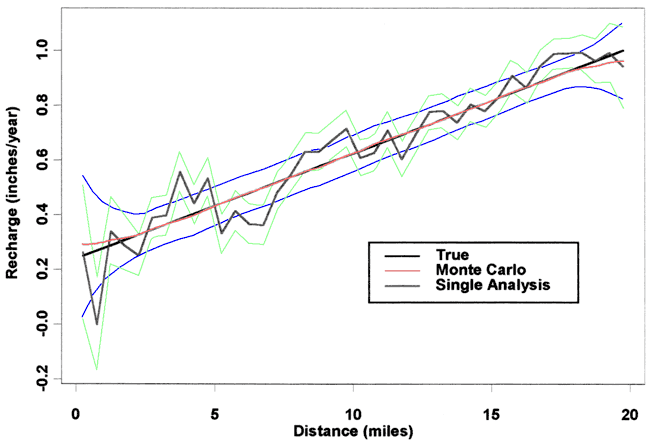
Increasing the number of points in the fitting window to 9 results in the data shown in Figure 6. Here the Monte Carlo results show that R is being estimated to within about plus or minus 10%. So, increasing the window length has helped considerably.
Figure 6. Scenario 1, σh of 0.1 ft, σk of 0.5 ft/day, 9-point fit.
If we increase the magnitude of the added Gaussian error to a σk of 5.0 ft/day and a σh of 1.0 ft, the results are shown in Figure 7 for a 9 point fitting window. Here the Monte Carlo results show that the recharge can not be estimated to better than about plus or minus 100%. The single realization for R has wide fluctuations about the correct value. The assumed error magnitudes used here are not as high as some that one might encounter in real systems. Therefore the implication is that it will be hard to estimate R in the presence of much error in h and K.
Figure 7. Scenario 1, σh of 1 ft, σk of 5 ft/day, 9-point fit.
Recharge scenario 2 has a linear trend going from 1/4 inch/yr to I inch/yr. The Monte Carlo results for a σk of 0.5 ft/day and a σh of 0.1 ft are shown in Figure 8 and indicate that the trend has been pretty well defined for this low error case.
Figure 8. Scenario 2, σh of 0.1 ft, σk of 0.5 ft/day, 9-point fit.
The third recharge scenario with two anomalies in a linear trend is estimated in Figure 9 for a σk of 0.5 ft/day and a σh of 0.1 ft and a 9 point fitting window. Again, the recharge has been reasonably well estimated for this low noise case. However, if we increase the error magnitudes to a σk of 5.0 ft/day and a σh of 1.0 ft, the results in Figure 10 show that the recharge profile is poorly estimated for this level of noise.
Figure 9. Scenario 3, σh of 0.1 ft, σk of 0.5 ft/day, 9-point fit.
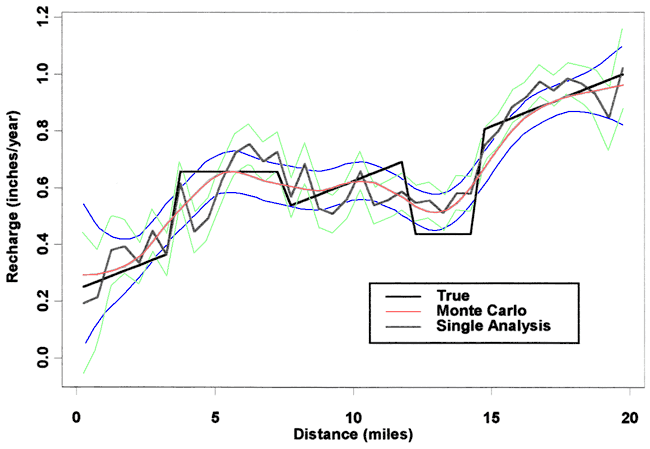
Figure 10. Scenario 3, σh of 1 ft, σk of 5 ft/day, 9-point fit.
We have investigated error propagation in steady state ground water models. We have considered normally distributed Gaussian errors with zero mean and a given standard deviation in the head and hydraulic conductivity profiles and have calculated their effect on estimation of the net model flux or recharge. Monte Carlo analysis has been used to generate statistics on recharge estimates and that result has been compared to the results from first order sensitivity analysis. The one standard deviation bounds calculated from the first order sensitivity analysis agree very well with the Monte Carlo results. However, the center points of these bounds are biased by whatever realization is used for R. It would appear that first order sensitivity analysis is fine for calculating the uncertainty bounds for any magnitude of error that yields a meaningful estimate of R. It appears the estimates of recharge are very sensitive to errors in head and hydraulic conductivity and can only be done with some confidence in low noise situations. Additionally, it appears that some level of averaging must be done even in the presence of low levels of noise. We have found that an averaging window of 5 to 9 node points is useful in suppressing noise. This means that it is unlikely that regional data on head and hydraulic conductivity can be used to infer the net aquifer flux or recharge on scales of less than several model node points.
Benjamin, J.R. and Cornell, C.A., 1970, Probability, statistics, and decision for Civil Engineers: McGraw-Hill Book Co., New York, 684 p.
Draper, N.R. and Smith, H., 1998, Applied regression analysis, Third Edition: John Wiley and Sons, Inc., New York, 706 p.
Hermance, J.F., 1999, A mathematical primer on groundwater flow: Prentice Hall, New Jersey, 230 p.
McElwee, C.D., 1987, Sensitivity analysis of ground-water models; in, J. Bear and M.Y. Corapcioglu (Editors), Proc. 1985 NATO Advanced Study Institute on Fundamentals of Transport Phenomena in Porous Media: Martinus Nijhoff, Dordrecht, pp. 751-817.
Sophocleous, M., 1998, Perspectives on sustainable development of water resources in Kansas: Kansas Geological Survey, Bulletin 239, 239 p.
Wang, H.F. and Anderson, M.P., 1982, Introduction to Groundwater Modeling: W.H. Freeman and Company, San Francisco, 237 p.
Kansas Geological Survey, Geohydrology
Placed online Nov. 27, 2007; original report dated June 1999
Comments to webadmin@kgs.ku.edu
The URL for this page is http://www.kgs.ku.edu/Hydro/Publications/1999/OFR99_20/index.html