Kansas Geological Survey, Open-file Report 83-6
KGS Open File Report 83-6
Read the PDF version (3 MB)
This investigation was conducted in order to evaluate the ability of surface electrical resistivity methods to distinguish areas of natural salt water intrusion in Groundwater Management District No. 5. Saline groundwaters are believed to leak from the subcropping Lower Permian age bedrock aquifer into the overlying Pleistocene and Recent-age unconsolidated aquifer in the eastern part of the District. This area was chosen for investigation because good subsurface control is available from a network of nested observation wells recently drilled in the District. The nested sets are spaced approximately six miles apart and each well nest consists of two or three wells completed at different depths in the subsurface. The deepest well in each nest is always completed in the Permian bedrock.
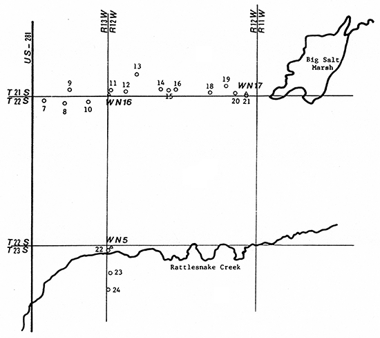
The study area is located in the northeast part of Stafford County (Fig. 1). Two lines of surface resistivity sounding stations were surveyed during this investigation (Fig. 2). The east-west line extends along the township line from one-half mile east of U.S. Highway 281 to within less than one mile of Big Salt Marsh. This line is made up of 14 (VES 7-20) vertical electrical soundings (VES). Also well nests WN16 and WN17 are located along this line. Three soundings (VES 22-24) were made along a north-south line extending south from WN5 across Rattlesnake Creek.
Figure 1--Study area in the northeast part of Stafford County.
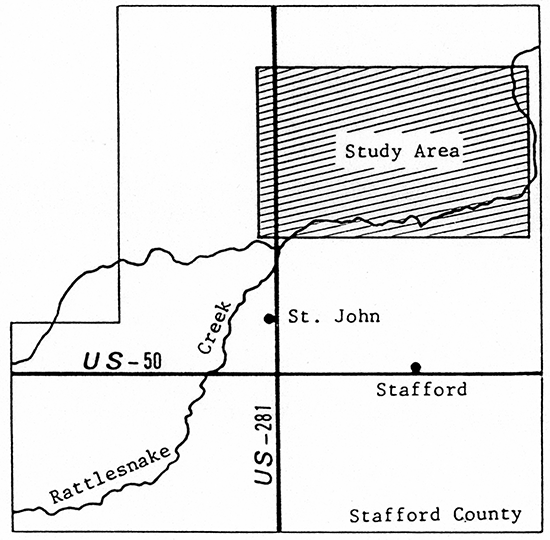
Figure 2--Locations of sounding stations.
The geology of the study area has been described in detail by Latta (1950) and updated by Cobb (1980). Unconsolidated deposits of Pleistocene and Recent age consisting of variable amounts of gravel, sand, silt, and clay cover the entire area. The total thickness of these deposits ranges from 114 feet (WN17) to 220 feet (WN16). These deposits rest unconformably on rocks of Lower Cretaceous or Lower Permian age. The surface trace of the contact between these two subcropping bedrock units lies between stations 9 and 10 and extends in a generally north-south direction across the study area (Fader and Stullken, 1978). The bedrock surface configuration beneath the unconsolidated deposits is quite irregular across the area. The Lower Cretaceous age units are undifferentiated, and consist of sandstones, shales, and siltstones of the lower part of the Kiowa Formation and the Cheyenne Sandstone. The Lower Permian age rocks are represented by redbeds consisting of fine-grained sandstones, shales, siltstones, and evaporites of the lower part of the Nippewalla Group.
The depth to the top of the salt water from land surface is known to vary considerably across the study area. Table 1 shows total solids levels of water samples collected from well nests in the study area.
Table 1--Total dissolved solids content of water samples from well nests WN5, WN16, and WN17. Data from Cobb (1980).
| Well Nest | Screened Interval From Land Surface (ft) |
Water Sample Total Dissolved Solids (mg/l) |
|---|---|---|
| WN5 Bedrock at 181 ft |
40-50 | 365 |
| 90-100 | 39,900 | |
| 193-198 | 74,600 | |
| WN16 Bedrock at 220 ft |
77-85 | 327 |
| 195-203 | 57,700 | |
| 240-248 | not available | |
| WN17 Bedrock at 114 ft |
40-46 | 440 |
| 100-107 | 16,500 | |
| 126-134 | not available |
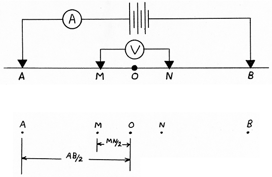
Vertical electrical soundings were made at each site using a Schlumberger electrode array (Fig. 3). Both an ABEM Terrameter and Bison Signal Enhanced Model 2390 resistivity measuring systems were used during the field work phase of the investigation. This was done to compare field performance of both systems, a secondary purpose for this investigation. Both units were used simultaneously at only two sites because of time restrictions. However, the Terrameter yielded results comparable to the Bison Instruments.
Figure 3--Profile and plan view of a Schlumberger array.
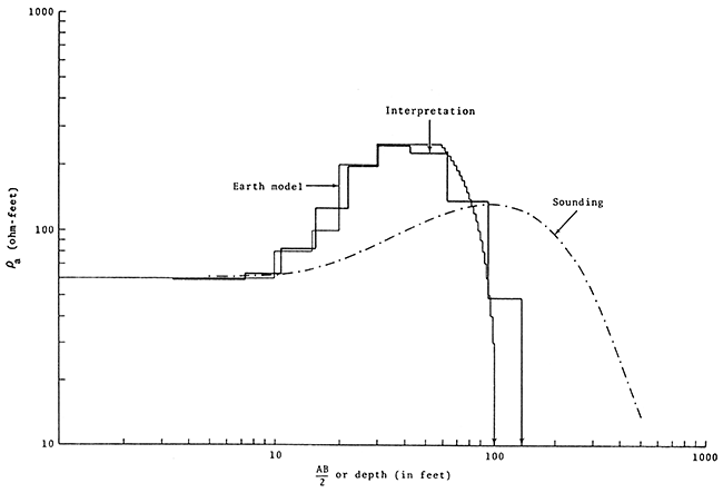
The data were plotted in the field on log-log coordinate paper as apparent resistivity, ρa, (ordinate) versus current probe spacing, AB/2, (abscissa) (see Fig. 4). The curve segments were then joined together holding the right-hand segment at the far end of the curve stationary and adjusting the others vertically up or down to form an unbroken curve. This procedure partially eliminates the effect of lateral inhomogeneities in the subsurface (Zohdy, et al., 1974). The resulting curves were digitized beginning at the right end and moving to the left at the rate of six equally spaced points per log cycle. The digitized data set (ρa, AB/2) was used as input into a modified version of Zohdy's (1973) computerized automatic interpretation program for Schlumberger soundings. Details concerning the automatic procedure can be found in Zohdy (1975). The output from this procedure is a computed earth model from the apparent resistivity curve composed of a sequence of geoelectric layer resistivities and thicknesses.
Figure 4--Apparent resistivity versus current probe spacing, VES11.
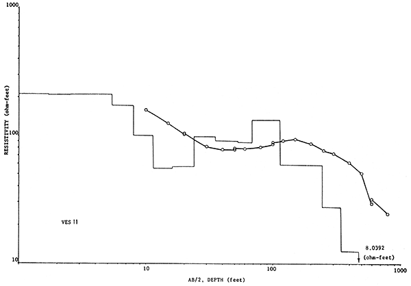
Table 2--Well log for the deepest well drilled at WN16, SW SW SW Sec. 31, T. 21 S., R. 12 W.
| Depth Below Land Surface (ft) | Lithologic Description | |
|---|---|---|
| From | To | |
| 0 | 5 | Sand top soil, yellow sand, fine to coarse |
| 5 | 8 | quartz arkose; yellow clay matrix |
| 8 | 35 | Sandy to silty clay, yellowish to greenish clay; some caliche |
| 35 | 140 | Sand, fine to coarse; gravel, quartz arkose |
| 140 | 160 | Sand, fine to coarse, quartz arkose |
| 160 | 165 | Silty clay, greenish gray |
| 165 | 220 | Gravel, fine to medium, quartz arkose; greenish-gray clay stringers |
| 220 | 248 | Sandy shale, red; top of the Permian at 220 feet |
VES20: VES20 was produced with an east-west oriented array adjacent WN17 (Fig. 5 and Table 3). Considerable discrepancies exist between the description of the unconsolidated sediments in the well log and a geologic interpretation of the layers in the upper part of the geoelectric sequence presented in Figure 5. This occurs because the relative effective thickness of the gravel layers is not sufficient for adequate detection by the resistivity method. The top of the fresh-salt water interface is interpreted to be 98 feet below the land surface.
Figure 5--Apparent resistivity versus current probe spacing, VES20.
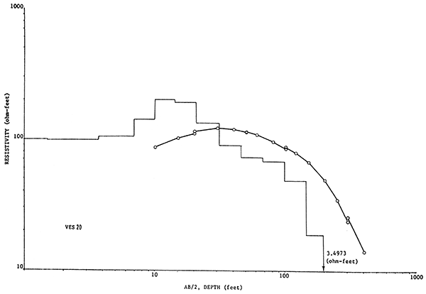
Table 3--Well-log of deepest well in WN17, SE SE SE Sec. 36, T. 21 S., R. 12 W.
| Depth Below Land Surface (ft) | Lithologic Description | |
|---|---|---|
| From | To | |
| 0 | 2 | Top soil |
| 2 | 40 | Clay, some caliche |
| 40 | 95 | Gravel, quartz arkose; clay matrix, tan |
| 95 | 97 | clay |
| 97 | 105 | Gravel, quartz arkose |
| 105 | 114 | Clay, tan with fine sand |
| 114 | 134 | Red siltstone; top of Permian at 114 ft |
VES22: VES22 is located approximately 1,500 feet south of WN5 near Rattlesnake Creek. The VES curve and layering are shown in Figure 6 and the well log of the site is tabulated in Table 4. The geoelectric model corresponds reasonably well to the well log for the site. Depth to the fresh-salt water interface is interpreted to be approximately 62 feet below land surface.
Figure 6--Apparent resistivity versus current probe spacing, VES22.
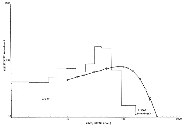
Table 4--Well-log of the deepest well in WN5, adjacent to Rattlesnake Creek, NW NW NW Sec. 6, T. 23 S., R. 12 W.
| Depth Below Land Surface (ft) | Lithologic Description | |
|---|---|---|
| From | To | |
| 0 | 3.5 | Silt, gray to brown |
| 3.5 | 61 | Sandy silt, orange-brown, fine grained, some blue-gray clay |
| 61 | 91 | Sand |
| 91 | 106 | Clay, tan |
| 106 | 150 | Clay, tan; sand, very fine, white |
| 150 | 181 | Sand, yellow, very fine-grained; trace of pink clay at 180 feet |
| 181 | 225 | Red mud; top of the Permian at 181 feet |
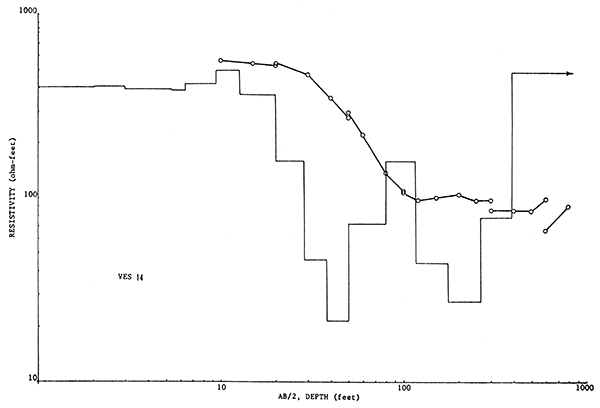
VES14: The layering of this site is different from all the others because the geoelectric basement (infinite layer) has a high true resistivity value relative to the resistivity values calculated for the basement at the other VES sites. This could probably signify the existence of highly resistive layers in the Permian bedrock or Cretaceous bedrock at depth below the unconsolidated sediments. However, laterologs from nearby oil wells do not indicate unusually resistive layers below the top of the Permian until the Stone Corral Dolomite which is relatively thin. Because of this, it is difficult to evaluate this site in the context of soundings without additional work.
Figure 7--Apparent resistivity versus current probe spacing, VES14.
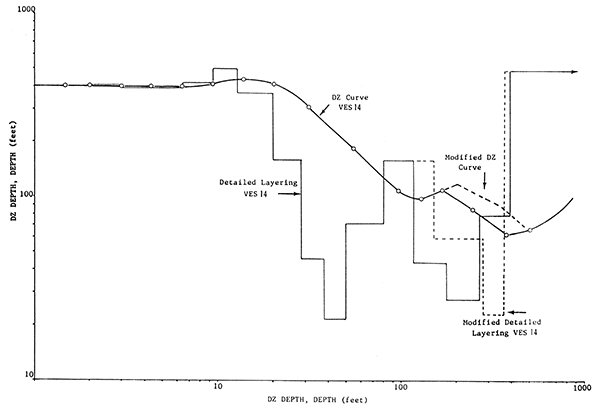
Studies of similar sites in Texas (Zohdy and Jackson, 1973) suggest that where highly resistive layers are below the top of the Permian, the top of the shale cannot be discerned without additional information. However, by interpolating between VES13 and VES15 some modifications in the interpretation can be made by changing the Dar Zarrouk curve for VES14 shown in Figure 8 (Zohdy, 1974b). It has been assumed that in the modified detailed layering the 161 ohm-feet layer extends to a depth of 150 feet. Below are two layers of 60 and 23 ohm-feet, respectively. The second and third layers in the modified sequence represent unconsolidated sediments and Permian shale containing saline waters, respectively, and the resistive layers are 84 feet below the top of the Permian bedrock. The modified layering seems to fit the geology better than the original sequence of layers in the detailed interpretation. The highly resistive layer is shifted upward slightly and is now 84 feet below the subcropping shale. No comparisons were made between the original and modified soundings to check for equivalence and no additional work was done to field verify the apparent resistivity curve for this site.
Figure 8--Modification of curve for VES14 using info from VES13 and VES15.
Much better estimates of the depth to bedrock and the fresh-salt water interface can be made from cross-sections showing a contoured distribution of true resistivity than from an evaluation of a geoelectric sequence at a site. It is assumed in this method that resistivity varies continuously vertically and horizontally. The mid-point of each layer in the earth model for each VES site is plotted on the cross-section and assigned the true resistivity for that layer. The cross-section can then be contoured and interpreted. Each contour represents a line of equal resistivity (isoresistivity) on the cross-section. Relatively low resistivity areas on the cross-section generally correspond to fine-grained unconsolidated sediments and bedrock or areas containing relatively saline groundwaters. Areas of the cross-section showing relatively high resistivity correspond to coarser-grained unconsolidated sediments and bedrock, evaporites, dolomite or relatively fresh water. Depth to the top of the Permian shale was interpreted to coincide with the 50 ohm-foot contour on cross-section VES7-VES20 from the drill hole.
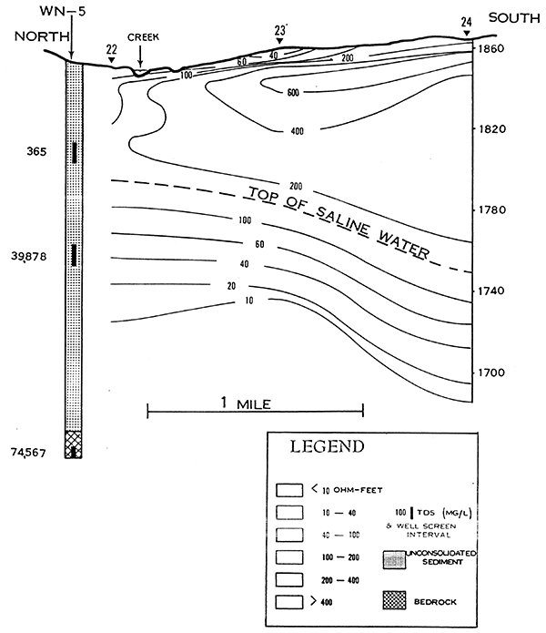
Cross-Section VES22-VES24: This line of cross-section extends in a north-south direction across Rattlesnake Creek and was constructed from VES22, 23, and 24 (Figs. 2 and 9). Rattlesnake Creek is located just south of VES22 and WN5 is located north of this site. The zone of relatively saline water represented on the cross-section by the set nearly parallel contours in the lower portion of the aquifer. The top of "saline" water is located midway between the 100 and 200 ohm-feet contours and becomes shallower underneath Rattlesnake Creek, a phenomenon observed by Cobb (1980). The depth to the top of the bedrock cannot be interpreted from data available because the resistivity contrast between bedrock and brine-saturated unconsolidated aquifer is too low.
Figure 9--North-south cross-section VES22-VES24.
Cross-Section VES7-VES20: The line of cross-section extends from one-half mile east of US 281 eastward to the edge of the Big Salt Marsh. Fourteen vertical electric soundings were used to construct the cross-section (Figs. 2 and 10). WN16 and 17 are located on the figure which includes the total dissolved solids concentrations for water samples from the wells in each nest. The top of the Permian shale and the top of "saline" water have been interpreted from the contoured cross-section and are also indicated.
Figure 10--East-west cross-section VES7-VES20.
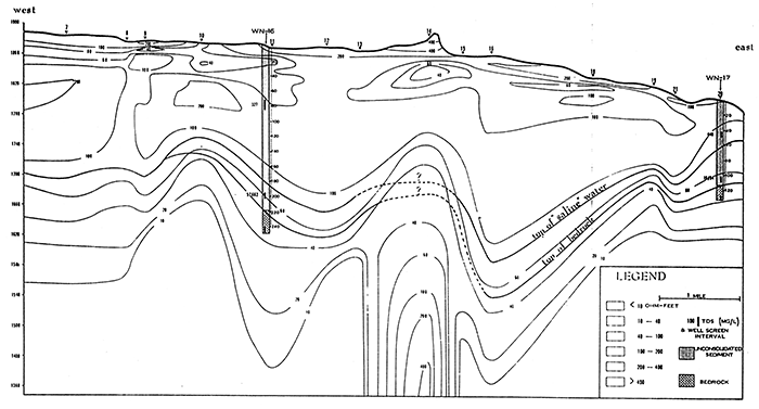
Several features are generally depicted by the configuration of the isoresistivity contours on the cross-section. Most of the shallow (less than 20 ft) subsurface is composed of relatively high-resistivity unconsolidated material, probably dry sand or silt. Below this shallow zone are low resistivity (100 to 20 ohm-feet) layers which are interpreted to be fresh water saturated fine sand, silt, or clay. These materials are about 40 to 50 feet thick across most of the cross-section and appear to be particularly clayey under VES14, 15, 8, 9, and 10. This low resistivity zone is underlain by a zone of higher resistivity (100 to 215 ohm-feet) interpreted to be freshwater saturated sand and silt. Saline water bearing materials begin below the line indicating the top of the "saline" water, midway between the 60 and 100 ohm-feet contours. The line representing the top of bedrock was drawn on the cross-section following the approximate position of the 50 ohm-feet contour at the base of the cross-section. The locations of the top of bedrock and the top of saline waters below VES14 are inferred.
The position of the top of "saline" water line is somewhat arbitrary even though it was determined using the groundwater chemical quality information available from the well nests. This is because the interface between fresh and salt water in the unconsolidated aquifer is not a sharp interface, but is actually a vertically diffuse zone (Cobb, 1980). However, from working with simple geoelectric models containing transition layers it appears to be fairly easy to distinguish the top of the transition zone in the subsurface with apparent resistivity data. Figure 11 shows a geoelectric earth model containing a simulated transition "layer" where the bulk resistivity of the "layer" changes linearly with depth from 250 ohm-feet at the top to 50 ohm-feet at the bottom. The 45-foot thick transition layer has been simulated a sequence two foot thick layers. The bulk resistivity of the infinite layer is 5 ohm-feet. Also shown are the simulated apparent resistivity curve computed from the forward calculation program of Zohdy (1974c) and the resulting layering computed from this simulated curve. The detailed layer model over estimates the top of this transition by four feet. Notice that the apparent resistivity curve is similar to the field curves produced along Rattlesnake Creek.
Figure 11--Geoelectric earth model containing a simulated transition "layer".
An attempt was also made to determine the relationship between the vertical distribution of porewater, total dissolved solids, and bulk resistivity computed from the sounding curves within the transition zone. This was not successful for several reasons. First, the Archie formation factor is not a constant in the subsurface, but is spatially variable. This is quite evident from the well logs of each of the well nests. Secondly, it appears unlikely that the surface resistivity method could discern differences between the possible relationships governing porewater resistivity with depth even if the formation factor were constant. Koefoed (1979) points out that without other subsurface data, such as from drilling, the presence of a transitional layer cannot be detected because the transitional layer will be replaced with an electrically equivalent sequence of thinner homogeneous layers. Furthermore, the vertical changes of resistivity in the transition zone cannot be calculated unless the mathematical relation between resistivity and depth is known in advance. We have found that unless the thickness of the transition layer in a three layer earth model is substantially greater than that of the overlying layer, the effect of changing the distribution of resistivity in the transition is almost negligible on the apparent resistivity curve. We conclude, therefore, that under natural conditions the surface resistivity method cannot be used to map variations in porewater dissolved solids within fresh-saltwater transition zones.
The surface resistivity method seems to be quite useful for determining the depth to the top of the fresh-salt water interface in the Great Bend Prairie, especially if additional geologic and groundwater chemical quality data are available. However, it was difficult to interpret the position of this interface at VES14 where highly resistive layers are present near the interface. In this situation, additional drill-hole information is necessary for valid interpretation. Generally, the method cannot distinguish between brine saturated zones in the aquifer and the Permian shale. because the geoelectric contrast between these two materials is not generally sufficient. However, in this case the top of the Permian shale was interpreted from the drill-hole data to coincide with the 50 ohm-feet contour. It is unlikely that the surface resistivity method can be used to map variations in total dissolved solids within the transition zone.
Cobb, P.M., 1980, The distribution and mechanisms of salt-water intrusion in the fresh-water aquifer and in Rattlesnake Creek, Stafford County, Kansas: Unpublished M.S. thesis, The University of Kansas, 176 p.
Fader, S.W. and Stullken, L.E., 1978, Geohydrology of the Great Bend Prairie, south-central Kansas: Kansas Geological Survey Irrigation Series 4, 19 p. [available online]
Koefoed, O., 1979, Geosounding principles, 1: resistivity sounding principles: Methods in Geochemistry and Geophysics, 14A: New York, Elsevier, 170 p.
Latta, B.F., 1950, Geology and ground-water resources of Barton and Stafford counties, Kansas: Kansas Geological Survey Bulletin 88, 228 p. [available online]
Zohdy, A.A.R., 1973, A computer program for the automatic interpretation of Schlumberger sounding curves over horizontally stratified media: U.S. Department of Commerce, NTIS, USGS-GD-74-017, PB232 703, 31 p.
Zohdy, A.A.R., 1974a, Application of surface geophysics to ground-water investigations, electrical methods: U.S. Geological Survey Techniques of Water Resources Investigations, Book 2, Chapter D1, 116 p. [available online]
Zohdy, A.A.R., 1974b, Use of Dar Zarrouk in the interpretation of vertical electrical sounding data: U.S. Geological Survey Bulletin 1313-D, 41 p. [available online]
Zohdy, A.A.R., 1974c, A computer program for the calculation of Schlumberger sounding curves by convolution: NTIS, USGS-GD-74-010.
Zohdy, A.A.R., 1975, Automatic interpretation of Schlumberger sounding curves using modified Dar Zarrouk functions: U.S. Geological Survey Bulletin 1313-E, 39 p. [available online]
Zohdy, A.A.R. and Jackson, D.B., 1973, Recognition of natural brine by electrical soundings near the Salt Fork of the Brazos River, Kent and Stonewall counties, Texas: U.S. Geological Survey Professional Paper 809-A, 13 p. [available online]
Kansas Geological Survey, Geohydrology
Placed online Feb. 21, 2017
Comments to webadmin@kgs.ku.edu
The URL for this page is http://www.kgs.ku.edu/Hydro/Publications/1983/OFR83_6/index.html