J. A. Schloss
J. Mosteller
R. W. Buddemeier
B. A. Maxwell
J. D. Bartley
D. O. Whittemore
Note on Version 2.0 -- this version is unchanged from V1.0, but additional
related material has been added to
the Estimated Useable Lifetime section and the Water Table Drawdown
and Well Pumping appendix to the Atlas (Part A of this report).
| Contents | ||
|---|---|---|
| Introduction | ||
| 1. Water level changes determined from wells with long-term records | ||
| 2. Short-term water level changes determined from all available well records | ||
| 3. Areal extent and uncertainty
of depleted and endangered regions
See also Estimated Useable Lifetime section, Part A (Atlas) |
||
| 4. Symptoms and sources of uncertainty in water level data | ||
| 5. Identification of aquifer sub-units for analysis and management |
Introduction
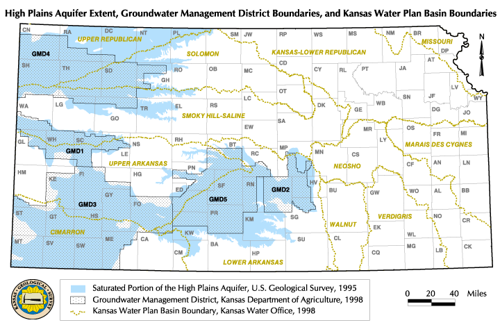
The Ogallala Aquifer is the western portion of the High Plains Aquifer (from the Colorado border to approximately the eastern boundary of Ford County). This portion of the aquifer has the lowest recharge and the greatest changes in saturated thickness, and in most areas is managed under "programmed depletion" rather than "safe yield" policies. One of the Kansas Water Plan Objectives for the region is "By 2010, reduce water level decline rates within the Ogallala Aquifer and implement enhanced water management in targeted areas." Under House Substitute for Senate Bill 287, the KWO has been charged to "...study and develop recommendations related to aquifer resources, recharge rates, availability of surface water resources and the long-term prospects related to any necessary transition to dryland farming in areas of the state to maintain sustainable yield and minimum streamflow levels." Central to both of these goals is an understanding of aquifer decline rates, the accuracy and precision with which they can be determined, and the determination of how to identify and 'target' critical areas.
The first two sections of this report present calculations of the average rate of change in saturated thickness in the Ogallala Aquifer as a whole, and in the Groundwater Management Districts and the portions of the river basins (see map) overlying the aquifer. Two different approaches were used: one employed data from those wells that had 30 years of measurement record, and the other used all available measurements over the past 11 years. Although neither of the methods of determination were identical to the calculations used to produce the maps in the atlas section (2000-29A) of this report (see note on methods and qualifications below), the general agreement among the results validate the overall findings and provide some comparison of the rates of change at different periods of time. The results indicate a level of temporal (rate) uncertainty in water level changes that is large compared to the precision desirable for meeting the specified goals.
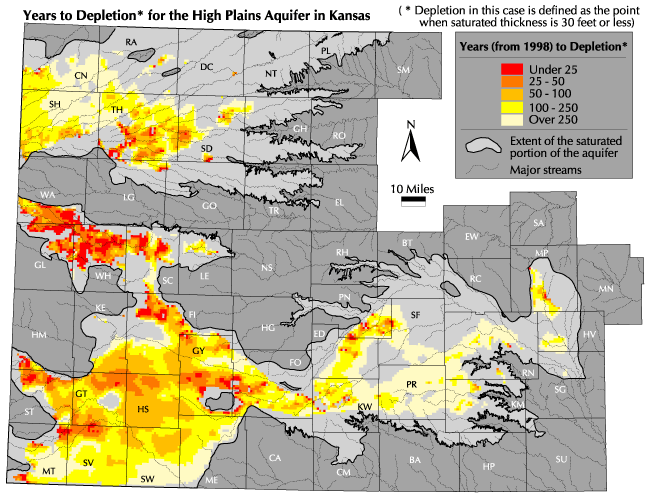
The third section integrates these findings with the 'time to depletion' product of the High Plains atlas, and with follow-up developments of that original data set. This section addresses issues of spatial uncertainty stemming from present applications of the available data, which compound the problem of temporal uncertainty.
Section 4 presents some initial assessments of individual well measurement uncertainties, and outlines efforts presently underway to identify their sources and possible approaches to improving measurement accuracy and precision.
The final section addresses issues of identifying aquifer sub-units that might be more appropriate to targeted management than are boundaries based on legal units (e.g., townships) or surface water features such as river basins. It considers both the implications and indications of some of the findings of the Atlas section of the report, and presents an initial trial application of a new geospatial clustering software package to aquifer data related to time to depletion.
Average values for the regions of interest were calculated both arithmetically and with area-weighting by Theissen polygons. Values are contained in the MS Excel summary file. The multi-year, area-weighted approach is considered the most robust and defensible, and was used to develop the figures shown below.

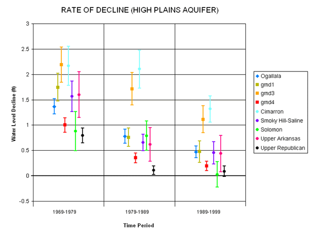
Results: The figures show three major results: (1) rates at which the various regions of the aquifer are declining have generally slowed substantially between the 1969-79 and 1989-99 periods; (2) the changes in the 1979-89 decade are not consistent across the various sub-units; and (3) the pattern and amount of change observed is strongly dependent on the region considered.
Methods and qualifications: The estimates in these figures were produced by averaging the ten-year changes in wells that had measurements in each of the years defining the endpoints of the decades. This method results in more precise individual values, but a much smaller number of wells -- and therefore greater uncertainty as to how well their average represents the behavior of the overall region. In other words, only wells measured in the winters of 1969, 1979, 1989, and 1999 were used, but all of each wells' winter measurements were used in calculating the average for each year.
Another cautionary note is also expressed in the Atlas section on estimated usable lifetime; rates of decline may change either because the resource is being used more sustainably -- or because there is not enough left to use. Rate of decline figures needed to be considered in the context of the amount and distribution of the remaining resource; decreasing use in a fringe area (e.g., with 50' of saturated thickness or less) could mask more serious declines in the remaining resource if only averages are considered.
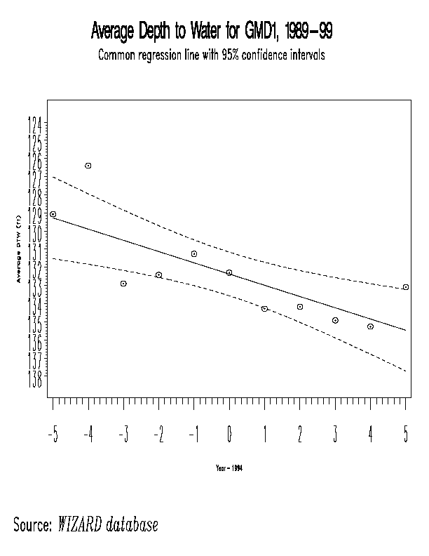
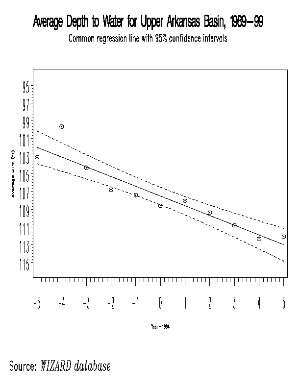
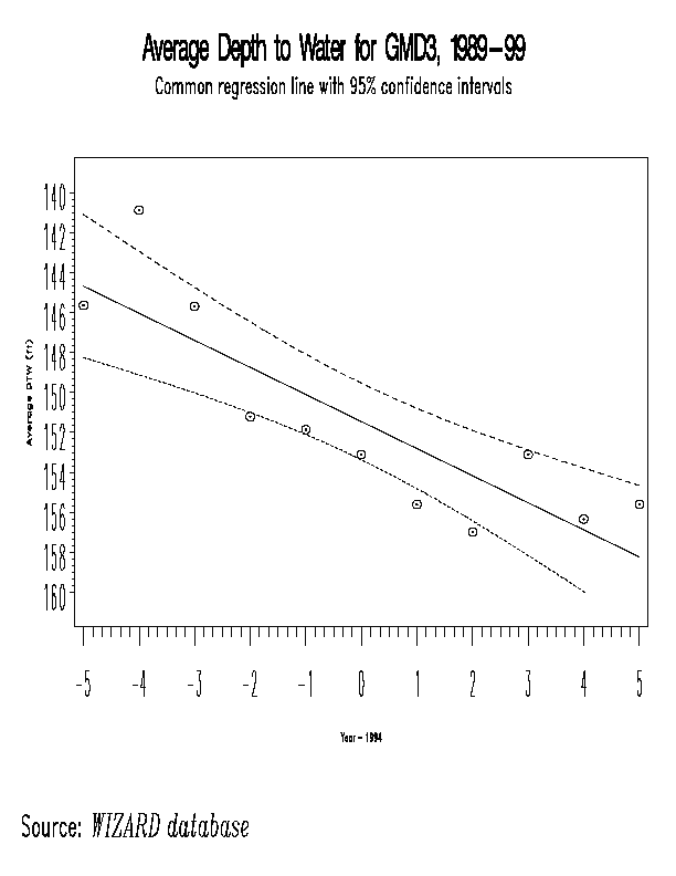
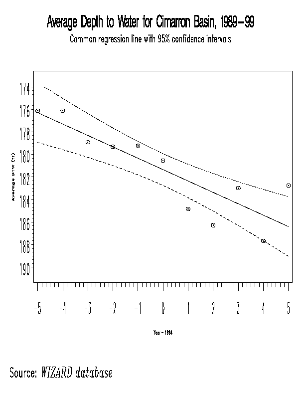
We would expect these values to be similar to those obtained in section 1 above for the 1989-99 decade (see right-hand column in figure 2). The general patterns are similar, but differ significantly in detail. Both methods find an average rate of decline of over a foot per year for southwestern Kansas GMD3 and the Cimarron basin, and agree on the small declines for the Solomon and Upper Republican basins. However, figure 2 shows a significant decline for the Smoky Hill-Saline basin and for northwestern Kansas GMD4, whereas Table 1 does not. Compared to Table 1, figure 2 underestimates the declines in the Upper Arkansas basin, western Kansas GMD1, and the Ogallala aquifer as a whole.
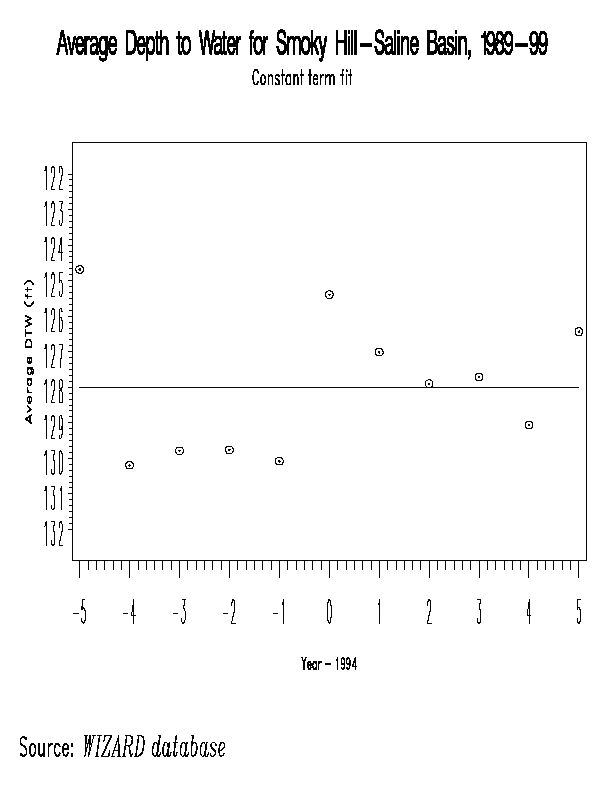
These values can then be compared with the time to depletion estimates (see Atlas section and section 3 below). The depletion time estimates are systematically different because they take into account saturated thickness, whereas the estimates discussed here simply address change in the elevation of the water table. The time to depletion map shows the greatest concentration of "hot spots" in GMD1, followed by the Smoky Hill-Saline basin and the Upper Arkansas basin. These findings, especially for the Smoky Hill-Saline basin, tend to generate very different management and planning perspectives than the values shown in Table 1 and figure 2
These differences can be resolved and explained by further analysis, but they point out the importance of developing clear, consistent measures of resource status and changes that take into account both hydrologic principles and the patterns of use.
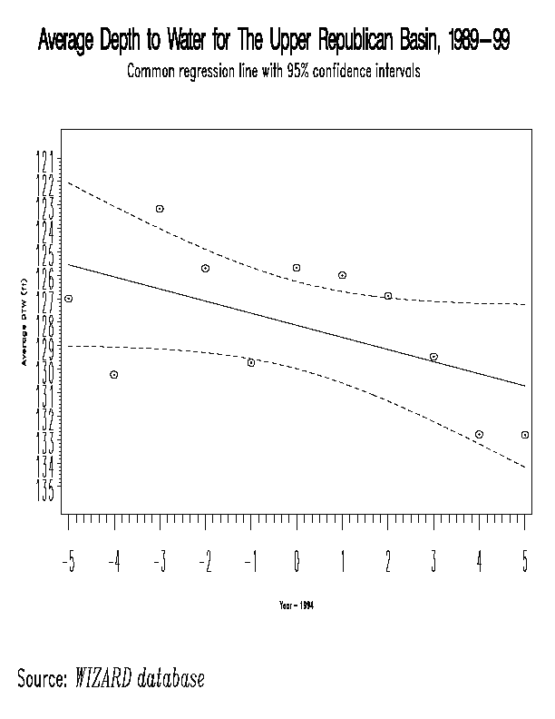
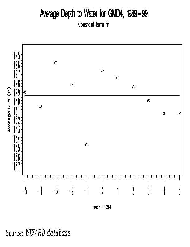
| Region | Average depth to water (ft) 1999 | Average rate of change (ft/yr) | Projected depth to water (ft), 2010 |
icance |
(gif) |
(.rtf) |
|---|---|---|---|---|---|---|
| Upper Republican | 132.81 | 0.326 | 136.40 | yes | rpub.gif | rpub.rtf |
| Solomon | 111.12 | 0.003 | 111.15 | no | solo.gif | solo.rtf |
| GMD4 | 131.37 | -0.171 | 129.49 | no | g4.gif | g4.rtf |
| Smoky Hill-Saline | 126.43 | 0.142 | 128.00 | no | smok.gif | smok.rtf |
| GMD1 | 133.09 | 0.836 | 142.29 | yes | g1.gif | g1.rtf |
| Upper Arkansas | 112.09 | 1.181 | 125.08 | yes | uark.gif | uark.rtf |
| GMD3 | 155.59 | 1.594 | 173.12 | yes | g3.gif | g3.rtf |
| Cimarron | 182.77 | 1.340 | 197.50 | yes | cimm.gif | cimm.rtf |
| Ogallala aquifer | 135.29 | 0.900 | 145.19 | yes | ogal.gif | ogal.rtf |
Methods and Qualifications: The data for each region were averaged for each year (1989-1999) and analyzed for trends; where a statistically significant change occurred, the "significance" column has a "yes". All significant trends were tested for best fit, and in all cases it was found that a linear trend line was better than any non-linear fit. The trend lines were then extrapolated to the year 2010 and an estimated value determined for that year.
These estimates make use of all available data rather than a limited subset of wells as is the case in the results reported in section 1 above. This should make the results more reliable, but the scale of the determinations in both cases is excessively large compared to the distribution of the resource and its uses. Averages therefore tend to smooth out the very real differences within regions, and paint the depleted, endangered, and relatively "safe" parts of the aquifer with the same brush. These results tend to support the need for developing appropriate techniques for classifying management and planning sub-units of the larger regions. The challenge inherent in this is that our databases put limits on the degree of local detail or precision that we can apply at smaller scales.
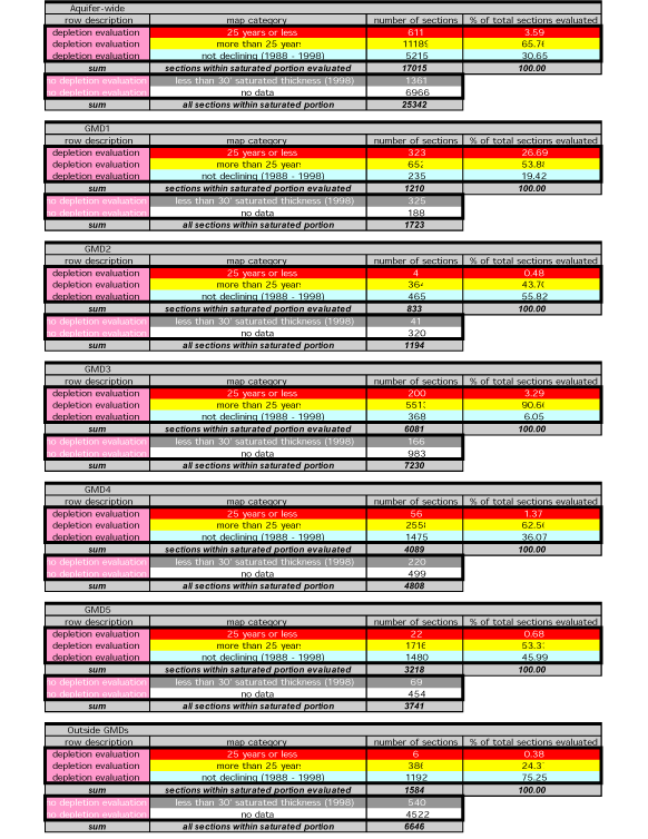
The Subcommittee on Water of the Vision 21st Century Task Force requested information on the percent of total area where time to depletion is less than 25 years. The following summarizes the development of the map and table that were produced in response. Concurrently, discussions with KDA-DWR staff identified the question of areas and locations of regions that are at risk of effective depletion of drawdown-induced impairment as in issue of priority concern (D. Pope, pers. commun.).
Development of Task Force Response
The interest was in the areas which would be first to be considered depleted, so the classification scheme seen on the public HPAE atlas web site was not used since it shows time-to-depletion classes that run up to the over 250 years. New class breaks were used that divided the sections as up into 25 years or less to depletion, and more that 25 years to depletion. A third class was added to show areas that were not declining (between the period 1987-89 and 1997-99). This class was not shown on the public atlas map since its intent was solely to show years to depletion, which could not be estimated for areas hat showed a recent water level rise.
Next, we wanted to some way be able to illustrate which sections for which a years-to-depletion estimate was not made. The reason for no estimate having been made was either because there were insufficient data to make a reasonably reliable estimate or because the area already had a saturated thickness of 30 feet or less, which by definition for this project was already depleted. Two classifications were added to the map and legend - one for areas with no data, and one for areas which had saturated thickness estimates of 30 feet or less.
Once the map classification scheme was worked out, we took all the relevant one-mile section data into Excel and calculated summaries for different the aquifer, each of regions, including the entire saturated portion of the five groundwater management districts, and areas within the aquifer but not within the boundaries of the groundwater management districts. We also calculated percentage of total area for each of the three classifications where a time to depletion evaluation was made. These were summarized in the table.
This classification scheme is more complex than the one used for the public atlas maps and yet it still does not fully describe every aspect of the dataset. For instance, the sections which had saturated thickness of 30 feet or less were not evaluated in terms of change from 1988-98 to determine if they might have increasing saturated thickness. If these areas are experiencing water- level rises they could potentially shed their depleted status. On the other hand, if they are still experiencing water-level declines, they could be reduced to having no saturated thickness. These areas, considered to be depleted at present, may deserve more attention than is given by the public atlas map which only classifies sections that are not yet depleted but are on the way; however, attempting to convey all the possible data classification schemes may warrant having more than one depletion map.
Analysis and Further Needs
When we examine the possibilities for estimating and communicating information about aquifer depletion, the classification schemes and the issues mentioned thus far pale in significance when we look at the various means of estimating risks or concerns associated with future depletion or recharge trends. For the High Plains atlas we used water- level data from two three-year periods set ten years apart. The variations that can be used are quite numerous - for example, instead of averaging over three-year periods, we could average the data over longer periods, or we could select different beginning and ending years for calculating water-level trends and arrive at very different estimates. We could also use data from every year in a given period instead of using three-year blocks at each end of the temporal range used to calculate the change in water level. These are but a few of the possible variations in data manipulation techniques.
An even larger issue is defining the real concerns to be addressed.
The table below summarizes some of the issues. If we look only at the area
of the aquifer showing < 25 years to depletion, we have 2.4% -- seemingly
a negligible fraction. However, an area more that twice as large already
has less than 30 feet of saturated thickness, so the total 'depleted' or
at risk is at least 7.8%. This fraction, however, is small compared to
the 27.5% of the aquifer for which we lack adequate data to make an estimate
-- and since much of this area is near the fringe of the aquifer, a substantial
fraction is probably close to the 30' criterion. Finally, 20.6% of the
aquifer had stable or rising water levels over the period 1989-1999. However,
much of this area is also near the fringe of the aquifer, and this was
an unusually wet period. If usage increased and/or recharge decreased in
these areas, some of them would be at risk of depletion. Depending on one's
projections of future climate and water use, anywhere from a quarter to
a half of the aquifer area might be considered at risk of depletion or
drawdown-based impairment.
| Category | Percent | Cumulative % |
|---|---|---|
| <25 years | 2.41 | 2.41 |
| Already <30' | 5.37 | 7.78 |
| Not evaluated | 27.49 | 35.27 |
| Not declining | 20.58 | 55.85 |
| >25 years | 44.15 | 100 |
This overview places the question in context -- an extremely optimistic view would conclude that only a negligible fraction of the aquifer is in danger of short-term depletion; an extremely pessimistic view would argue that as much as half of the aquifer is at risk. The truth almost certainly lies in between, but given the importance of the issues involved, this seems like an excessively large region of uncertainty.
Three factors need to be addressed:
4. Symptoms and sources of uncertainty in water level data
In order to assess the variability/uncertainty of water level measurements, analyses were performed on a subset of data on multiple measurement wells in the High Plains Aquifer region. The wells included in the database are ones in which there are multiple winter (Dec., Jan., Feb.) measurements for one of the benchmark years (1969,1979,1989,1999). The rate of change for the multiple measurement wells was determined by taking the difference between the highest and lowest water level measurements recorded within a season and dividing that by the number of days between measurements. This rate of change per day figure was then multiplied by 31 to obtain the rate of change per month. The degree of significant water level variability was taken as >0.25 ft per month. Since individual water level measurements are normally accurate to less than 0.1 foot, differences of a few tenths are readily measured. This magnitude of change rate, taken over the winter season of 2-3 months, would amount to a total change in excess of 0.5 feet. The average annual decline rate in most areas is a foot or less, so uncertainties of a significant fraction of a foot will seriously complicate determination of the decline rate and especially of changes in rate. Results are tabulated below.
Rates of water level change observed in wells with multiple winter season measurements in the indicated year
Year columns show number of wells and percent of the total with multiple measurements for each class
| Normalized rate of change (ft/mo) | 1969 | 1979 | 1989 | 1999 | total |
|---|---|---|---|---|---|
| <0.25 (not significant) |
|
|
|
|
|
| 0.25 (significant) |
|
|
|
|
|
| 0.5 (significant) |
|
|
|
|
|
| 1 (significant) |
|
|
|
|
|
| 1.5 (significant) |
|
|
|
|
|
| >2 (significant) |
|
|
|
|
|
| total | 57 | 47 | 24 | 20 | *148 |
| % of significant variation (>0.25 ft/mo) | 68.4% | 74.5% | 45.8% | 90% | 69.6% |
| * There are 148 multiple measurements distributed among 90 wells during the four selected years. | |||||
Geographic distributions are shown in the Western Kansas outline map below. The wells shown are those with multiple winter (Dec., Jan., Feb.) measurements for one of the benchmark years (1969,1979,1989,1999). Green = difference between measurements equivalent to a rate of change of < 0.25 ft/month. Yellow = difference between measurements equivalent to a rate of change > 0.25 ft/month.
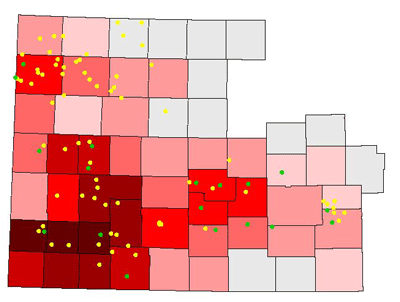
The background map for this figure indicates the relative number of acres within each county in the High Plains region that are typically planted in irrigated wheat. This number is normalized to a percentage in order to correct for the differences in area among the counties (acres irrig wheat in county / total acres in county). The counties are color coded from light red (lowest percentage) to dark red (highest percentage). Irrigated wheat may be a factor in the variability of water table measurements, since it is commonly irrigated later in the Fall than other crops, and may therefore result in incomplete well recovery in the vicinity. Another factor (not shown) under investigation is the possible influence of non-irrigation water rights (e.g., municipal wells) in proximity to the measurement wells.
If this sample is representative, it suggests that a majority of the wells measured in any year are not recovered, that the disequilibrium can be quite large, and that locations and magnitudes are not consistent. In order to use the results or short-term or small scale management, improvements are needed.
5. Identification of aquifer subunits for analysis and management
Background
Identification of appropriate units -- usually but not always geographically defined -- for resource assessment and management is a long-standing problem. Particularly in the case of groundwater, spatial and temporal distributions of the resource are difficult to detemine in detail, and often not consistent with human preferences for scales of operation.This section of the report explores initial approaches to hydogeologic definition of resource units, based on the following initial observations and premises:
The remainder of this report section explores the application of geospatial clustering techniques to the identification of regions of functional similarity within the High Plains Aquifer. Although the primary target is the Ogallala aquifer, the entire High Plains has been included in this initial analysis to explore similarities across the wider region. Subsequent analyses can focus on the regional or GMD level.
Methods
The LoiczView geospatial clustering package was used for the experiments described. It is a k-means clustering routine designed for high-dimensionality (multiple variables) data sets. Originally developed for analysis of coastal zone similarities at the global scale, it has been adapted and applied to vegetation and habitat studies as well as aquifer characteristics. It is described at the website (3) http://www.palantir.swarthmore.edu/~maxwell/loicz/, and in a manuscript submitted for publication in the journal Regional Environmental Change.
The data set clustered consisted of two variables for which section center coverages had been derived for essenially all of the High Plains aquifer. The annual water level trend is the average yearly rate of change in water level based on the analysis descibed in section 2 of this report (above). The 'feet to depletion' variable is the saturated thickness estimated at the section center minus 30' -- the estimated depletion threshold used in the 'time to depletion' section of the High Plains Atlas and this report. These variables contain the same information on which the original and modified time to depletion maps were based. However, the similarity analysis operates on the basis of natural classification of the data, rather than the imposition of classes defined in advance. For example, 25 years was picked as a key depletion time target. Without doing a series of remapping exercises we have no way of knowing whether a 30-year hreshold might include significantly more are or creat more continuous regions or potential management. Clustering the basic data and then evaluating the patterns provides a means of examining the questions.
Four clusters are shown here. Three illustrate the strategy of overclustering and then progressively merging the most similar clusters to explore patterns and relationships. These use the mean scaled Euclidian distance to distinguish the clusters, and are the results obtained for 12, 9 and 6 clusters. A fourth map was produced separately, using 5 clusters and the maximm scaled distance (see methods references for explanation of difference). All of the section-center cluster ID values were imported into ArcView from the LoiczView visualization package and mapped to provide comparability of the intervals defined.
Results and discussion
A composite of the maps obtained is shown below.
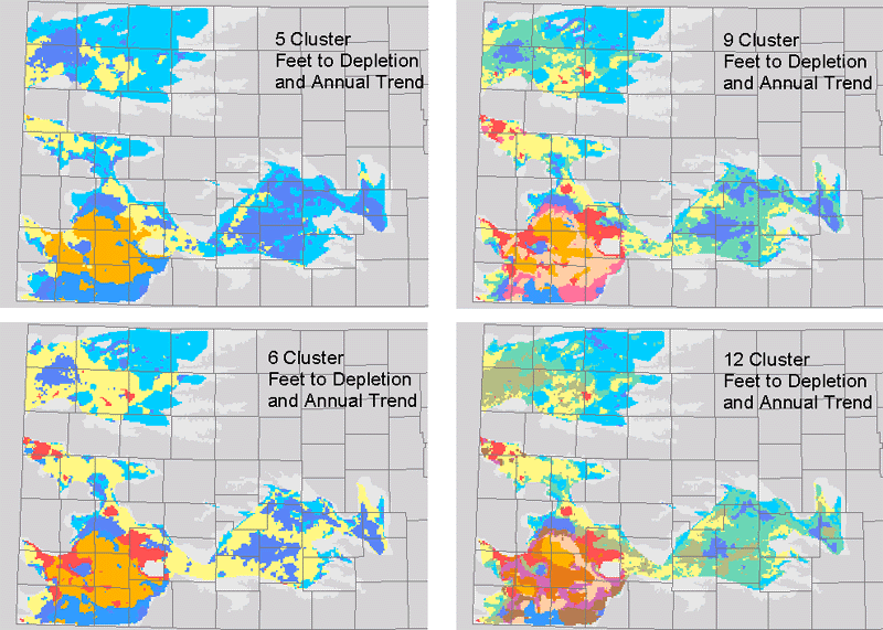
Comparison of the smaller numbers of clusters with the time to depletion maps shows a strong similarity of pattern, with some useful differences.
 |
 |
Patterns are clearly basically similar (as expected), but the clustering
classsifies as similar regions that appear quite distinct when the somewhat
arbitrary time classes are imposed. This is an important finding, since
it suggests that there may be hydrologic reasons for applying similar assessment
and management techniques across regions that might be considered separate
if viewed from a strictly regulatory perspective. More importantly, clustering
provides an objective basis for considering similarities over a much wider
range of variables than can conveniently be mapped individually or analytically.
See also: estimated usable lifetime, current maximum authorized use, current saturated thickness, groundwater availability and accessibility
Funded (in part) by the Kansas Water Plan Fund