KGS--OFR 2001-17--Electromagnetic Method to Locate Abandoned Brine Wells--Final Report

Kansas Geological Survey, Open-file Report 2001-17

Using the Electromagnetic Method to Locate Abandoned Brine Wells in Hutchinson, Kansas

by Jianghai Xia
Kansas Geological Survey
1930 Constant Avenue, Campus West
Lawrence, KS 66047

Final Report
KGS Open File Report 2001-17
May 2001

Summary

An electromagnetic (EM) survey with a GEM-2, an electromagnetic instrument, was conducted in Hutchinson, Kansas, as a part of effort to locate abandoned brine wells. EM results successfully located one uncapped abandoned brine well, 4 inches in diameter and buried at a depth of 5 ft. This survey result indicates the potential investigation depth with a GEM-2 would be as deep as 20 ft in locating abandoned wells in the Hutchinson area. The survey also demonstrated the importance of acquiring target signals in interpreting anomalies. The results of EM survey in Hutchinson demonstrated successfulness and effectiveness in locating the abandoned brine wells.

Introduction

On January 17, 2001, a natural gas explosion and fire destroyed two downtown Hutchinson businesses. The next day at a mobile home park 3 miles away, another explosion occurred. Two residents died of injuries from the explosion, which forced the evacuation of hundreds of people as gas geysers began erupting in the area. The geysers spewed a mixture of natural gas and saltwater. The pathways to the land surface at both the explosion sites and the geysers were abandoned brine wells used for solution mining of salt (http://www.kgs.ku.edu/Hydro/Hutch/Background/index.html).

To find these abandoned brine wells is a part of the Hutchinson Response Project. Hutchinson City and state officials estimate that there may be more than 160 abandoned brine wells in and around Hutchinson. It costs about $60,000 to plug an abandoned well (Hutchinson News, May 9, 2001).

Some known wells in the mobile home park had steel cased pipes (Figure 1). A microgravity survey was not proposed to locate abandoned brine wells because anomalies due to brine wells or salt voids are too weak to be detected by this method. The length of vertical steel pipe normally is 400 - 700 ft. The predicted maximum gravity signal caused by this pipe is only 4 - 6 microGal). The sensitivity of the most advanced gravitymeter is at a one microGal level so this anomaly is too weak to find using microgravity survey. I also calculated the gravity anomaly caused by a salt cavern with a volume of 100 ft x 100 ft x 100 ft buried at a depth 400 ft, a typical depth of salt voids in Hutchinson area. The maximum anomaly from the cavern is approximately 25 microGal, assuming that the cavern is completely empty. In actuality, the maximum anomaly due to the cavern will be much less than 25 microGal because caverns are always filled with water, soil, and/or rocks, which makes a density contrast considerably smaller. To detect this 25-microGal anomaly, sensitivity of the gravitymeter and accuracy of elevation measurements are critical. The sensitivity of the most advanced gravitymeters available in the market is 1 to 10 microGal. It takes much longer (normally more than 15 minutes/station) to acquire a microgravity data than a normal exploration gravity survey in order to achieve the 1-microGal sensitivity level.

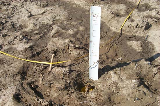
Figure 1. Well 8C, an abandoned brine well, cost two people their lives.

photo of abandoned brine well

Elevation measurements are the other main challenge in the microgravity survey. The error associated with elevation measurements is 5 microGal per inch. In practice, one inch accuracy could be achieved by the most advanced Trimble GPS system.

To confidently identify a gravity anomaly, the maximum anomaly should be at least three times higher than possible errors. Therefore, to see an anomaly with an amplitude less than 25 microGal, the sensitivity of gravitymeter should not be less than 4 microGal (in the range of 1-4 microGal) and the accuracy of elevation measurements should be within one inch. It is very difficult to achieve an accuracy of elevation survey with one-inch range. In addition, to detect this 25-microGal anomaly in an urban area, culture noise will become a serious problem.

A 3-D ground penetrating radar (GPR) survey may be useful to locate these wells. The ground is dirt fill, however, and there could be a lot of reflected/diffracted events caused by objects other than the brine wells. Furthermore, time spent on 3-D GPR data acquisition and processing could be much longer than might be expected.

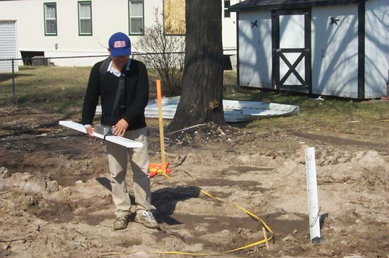
I proposed to use the eletromagnetic (EM) method to search for wells. A GEM-2 (Figure 2) is an EM instrument that can survey an area quickly and with great detail (Won, 1980). Data can transferred into a notebook computer and maps generated within a few minutes after the survey is done. The GEM-2 is a portable, digital, broadband electromagnetic sensor. Multi-frequency data are acquired simultaneously with a maximum sampling rate of 30 Hz when an instrument operator walks along a survey line. For each frequency, both in-phase and quadrature components of the induced EM field in ppm (parts per million relative to the primary field) were recorded.

Figure 2. EM survey with a GEM-2.

photo of GEM2 in operation

The measured in-phase and/or quadrature responses can be used to calculate apparent conductivity and apparent magnetic susceptibility based on a homogeneous half-space assumption by Won et al. (1996 and 1997). Apparent conductivity and apparent magnetic susceptibility are parameters that in general are related to targeted electrical and magnetic properties. Calculation of apparent conductivity and apparent magnetic susceptibility is a method of normalization of the EM data; it makes data analysis and interpretation easier for both geophysicists and other scientists. If the earth were truly homogeneous, the apparent conductivity would be the same at all frequencies and equal the true earth conductivity data (Huang and Won, 2001). In the real world, conductivity measurements are "bulk" or apparent conductivity. We will omit a word "apparent" from now on.

Quadrature data are proportional to the ground conductivity in the low to middle induction numbers, but are inversely proportional to the conductivity at middle to high induction numbers. Thus, a moderate conductor may produce a strong quadrature anomaly, whereas a good conductor may produce a weak anomaly or no anomaly. In either case, in-phase data have to be used for further analysis (Huang and Won, 2001). An anomaly shown on conductivity maps should also show on in-phase and/or quadrature data. The investigation depth is dependent on the frequency of the instrument used in the survey, conductivity and magnetic susceptibility of a target and surrounding materials. There is no exact relation between instrument frequencies and the investigation depth. A skin depth concept (Won, 1980) may be used to obtain rough estimates of the investigation depth in a specific survey area.

An EM survey was conducted in the open field on the southwest corner of 11th and Chemical Streets (Xia, 2001). Four anomalies were identified and reported. Anomaly four was caused by an abandoned brine well, 4 inches in diameter and buried in 5 ft deep. The first three anomalies were discussed in Xia (2001).

Methodology

Three frequencies were chosen for this project: 2,430 Hz, 7,290 Hz, and 18,270 Hz. For each frequency, both in-phase and quadrature components of the induced EM field in ppm were recorded. EM signals from a known well were first recorded to determine what kind of anomaly would be identified as a possible buried well. The signals then were compared with EM reconnaissance results acquired on an assigned area. To acquire signals from a known well was important for interpretation of anomalies. Signals from abandoned wells are dependent on a physical size of wells, buried depth, surrounding materials, and most importantly, calibration of an individual instrument.

EM signals from Well 8C

Well 8C is the well that costs two people their lives (Figure 3). I acquired GEM-2 data on an area 18 ft by 18 ft along lines with 2 ft spacing (Figure 4). Well 8C is located at point (19, 17). The signals from the well are all ellipses in both in-phase and quadrature components (Figures 5a - 5f). A positive anomaly in the southeast corner is caused by rebar in the driveway. Amplitudes of signals with 2,430 Hz from the well are much higher than signals with the other two frequencies (Table 1).

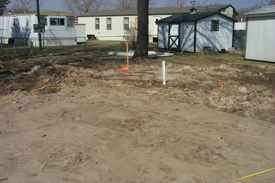
Figure 3. An EM survey grid is centered at Well 8C.

Well 8C

Figure 4. Arrows indicate the walking direction.

Pattern of data acquisition.

Well 8C--Click on figures to view larger versions

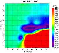
Figure 5a. 2430 Hz in Phase.

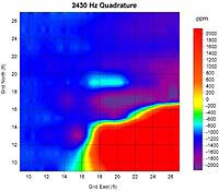
Figure 5b. 2430 Hz Quadrature.

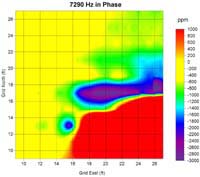
Figure 5c 7290 Hz in Phase.

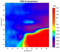
Figure 5d 7290 Hz Quadrature.

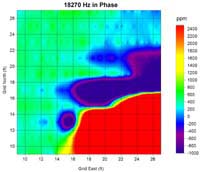
Figure 5e 18270 Hz in Phase.

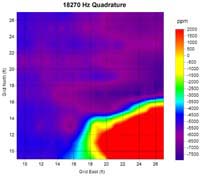
Figure 5f 18270 Hz Quadrature.

Table 1. Amplitudes (in ppm) of EM signals from well 8C.

2,430 Hz (I) 2,430 Hz (Q) 7,290 Hz (I) 7,290 Hz (Q) 18,270 Hz (I) 18,270 Hz (Q)

1,700 1,200 2,500 1,700 2,700 2,000

Well 8C--Click on figures to view larger versions
Figure 5a. 2430 Hz in Phase.	Figure 5b. 2430 Hz Quadrature.
Figure 5c 7290 Hz in Phase.	Figure 5d 7290 Hz Quadrature.
Figure 5e 18270 Hz in Phase.	Figure 5f 18270 Hz Quadrature.

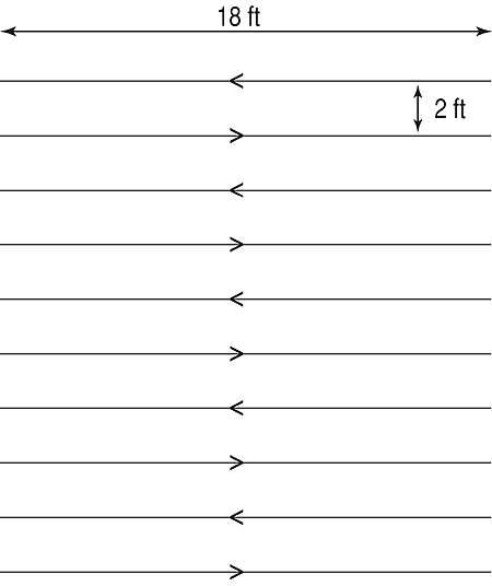
I expected to see a bulls-eye shape anomaly from the well. The anomaly shown in Figure 3 is in an ellipse shape with a longer axis in an east-west direction. I walked along an east-west direction with a GEM-2 oriented in the same direction. The sample point is about 2 ft away from the receiver coil. Data recorded along each line were linearly interpolated based on the starting point and the ending point when generating Figures 5a-5f. Therefore, I believe that the ellipse-like anomaly caused by well 8C instead of a bulls-eye anomaly is due to the way I acquired data and the 6-ft distance between a transmitter coil and a receiver coil of a GEM-2. The 6-ft distance between a transmitter coil and a receiver coil of a GEM-2 is also a criterion of a horizontal location of an anomaly object. Based on the results from well 8C, I would conclude that half the distance between a transmitter coil and receive coil (3 ft) of a GEM-2 might be an estimated accuracy of the horizontal location of an anomaly object. The elliptical effect due to the 6-ft coil distance and the way of walking along lines will be reduced when lines are much longer than the testing grid at well 8C. Thus, bulls-eye anomalies are my main objectives in locating abandoned brine wells.

When using the signals to compare data from an assigned area, two other characters may be changed. The depth of a well header affects the size of a bulls-eye and amplitude of signals. The deeper the well, the broader (in horizontal dimensions) the bulls-eye and the lower the amplitude will be. Abandoned wells were normally buried 3-4 ft under the ground. The signals from well 8C are from a well header on the ground. Thus, the bulls-eye anomalies from buried wells should be broader than the bulls-eye (Figure 5) from well 8C with a normally lower amplitude.

With a different GEM-2 instrument, different signals, polarity and amplitude, may be acquired on the same site due to calibration of the instrument. Thus, it is important to obtain signature readings from something that is known to be what the survey is looking for.

EM Survey Results on the Southwest Corner of 11th and Chemical Streets

A 200 ft by 180 ft grid was surveyed on the southwest corner of 11th and Chemical Streets (Figure 6). Due to a data-storage limitation on the GEM-2, the EM survey was split into a south part (from 0 to 93 ft) and north part (from 93 ft to 180 ft). The EM survey was performed by walking along lines, with 3 ft between lines. (The survey was done the same as shown in Figure 4, except for the line spacing.) Total survey length is 12,000 ft. It took two persons 5 hours to lay out grids and to finish the EM survey. See Xia (2001) for details of survey results and discussion of anomalies identified from EM results.

Figures 7a - 7f present the south part of the GEM-2 results. The anomaly located at (110, 40) was not identified during anomaly verifications in the March trip (Xia, 2001). This anomaly showed a negative bulls-eye on all components except for the 18,270 Hz quadrature component (Figures 7a - 7f). Due to a target depth, it is expected that anomaly might disappear in higher frequency components. The 2,430 Hz results showed the highest amplitude in three frequencies (Table 2). Comparing Table 2 with Table 1, Xia (2001) interpreted that this anomaly to be caused by a buried well.

Table 2. Amplitudes (in ppm) of EM signals from anomaly at point (110, 40).

2,430 Hz (I)	2,430 Hz (Q)	7,290 Hz (I)	7,290 Hz (Q)	18,270 Hz (I)	18,270 Hz (Q)
2,800	1,400	3,600	700	3,600	n/a

Abandoned Brine Well Unearthed

A backhoe was on site during a May trip to Hutchinson. An uncapped abandoned brine well was unearthed beneath the point (110, 40) (Figure 8 and the cover photo). It is 4 inches in diameter and buried 5 ft in depth. Sandy soils, clay, and gravel are surrounding materials of the abandoned well.

To review Table 2, strong in-phase anomalies are shown in all three frequencies. A relatively strong quadrature anomaly is shown in the 2,430 Hz frequency results. This indicates that, based on the skin depth concept (Won, 1980), the investigation depth of a GEM-2 for a 4-inch well in diameter could be as deep as 20-30 ft in the Hutchinson area if frequencies around 1,000 Hz are used.

Conclusions

An uncapped abandoned brine well that is 4 inches in diameter and buried 5 ft in depth in Hutchinson was found by the electromagnetic method. The EM anomalies obtained by a GEM-2 suggests that the investigation depth by a GEM-2 in the Hutchinson area may be as deep as 20 ft. EM anomalies also indicated that it is critical to get a signature from a known well in order to identify anomalies that could be caused by an abandoned well. Results of the EM survey by a GEM-2 in Hutchinson were successful and effective in locating abandoned brine wells.

Acknowledgements

I greatly appreciate Dennis Clennan and Stephen William of the City of Hutchinson for their advice in locating the test site and Reg Jones, Kreg Luman, Robert Cape, Bill Stoy, and Chris Rucbke of the City of Hutchinson for their help in field operation. I thank Kyle Parker of the Kansas Department of Health and Environment and Sihao Xia of the University of Kansas for their assistant in data acquisition. I also thank Mary Brohammer for her efforts in preparation of this report.

References

Huang, H, and Won, I.J., 2001, Conductivity and susceptibility mapping using broadband electromagnetic sensors: Proceedings of the Symposium on the Application of Geophysics to Engineering and Environmental Problems (SAGEEP 2001), March 4-7, 2001, Denver, CO.

Won, I.J., 1980, A wideband electromagnetic exploration method--Some theoretical and experimental results: Geophysics, 45, 928-940.

Won, I.J., Keiswetter, D., Hanson, D., Novikova, E., and Hall, T. 1997, GEM-3: A Monostatic Broadband Electromagnetic Induction Sensor: Journal of Environmental and Engineering Geophysics, 2(1), 53-64.

Won, I.J., Keiswetter, D.A., Fields, G.R.A., and Sutton, L.C., 1996, GEM-2: A new multifrequency electromagnetic sensor: Journal of Environmental & Engineering Geophysics, 1, 129-137.

Xia, J., 2001, Feasibility study on using the electromagnetic method to locate abandoned brine wells in Hutchinson, Kansas: Kansas Geological Survey Open-file Report 2001-10.

Kansas Geological Survey, Geophysics
Placed online June 2001
Comments to webadmin@kgs.ku.edu
The URL for this page is http://www.kgs.ku.edu/Geophysics/OFR/2001/17/index.html