Kansas Geological Survey, Open-file Report 2001-7
by
Jianghai Xia, Thomas V. Weis, and Richard D. Miller
KGS Open File Report 2001-7
April 2001
Animal wastes normally produce materials with higher conductivity (Larson et al., 1997). Nearly 10,000 m of electromagnetic (EM) line surveys have been acquired around a hog confinement facility in western Kansas over the last three years. Approximately 5,500 m of data were acquired using a Geophex GEM2 instrument (in three frequencies) and 4,300 m of data were acquired using a Geonics EM34 instrument (in three coil separations). The purpose of the project has been to 1) find possible subsurface seepage around the hog lagoon and 2) evaluate two popular electromagnetic instruments in monitoring and/or detecting animal lagoon leakage and to set up an efficient field EM survey routine to monitor animal lagoon leakage. The first survey was carried out one week before the facility began operation in early 1999. The results of this survey provide a reference background of electromagnetic properties of the survey site. Additional surveys followed in the spring of 2000 and 2001. The general trends of electromagnetic properties over the last two years at this site are similar. No dramatic localized change is found when comparing results from all three years. Compared to the EM34, the GEM2 is a faster and easier instrument to operate. Maps of survey results from data collected with a GEM2 can be generated right after survey is done. This makes the GEM2 a timesaving instrument, especially in conducting 3-D EM surveys.
Large-scale hog facilities that house several thousand hogs can be found throughout the United States. Earthen storage lagoons are an integral part of the waste management and treatment system at many of these concentrated animal operations. The large concentrations of animals in small areas raise significant waste management issues because any seepage from a waste disposal lagoon could contaminate local groundwater sources (Parker et al., 1994).
Ham and Desutter (1998) used a water balance method to monitor seepage losses from hog-waste lagoons. Seepage was calculated as the difference between evaporation and changes in water depth during periods when no waste was added or removed from the lagoons. After talking with Prof Jay Ham at Kansas State University in early 1999, we proposed a feasibility study to use the electromagnetic method to monitor/detect hog lagoon leakage in Kansas. Prof Ham suggested a newly built hog facility in western Kansas as a test site (Figure 1).
Figure 1--Site map showing hog facility in Meade County, Kansas.
Electromagnetic (EM) surveying is a rapid field method and has been proved to be an effective tool in delineating leachate plumes emanating from animal waste lagoons (Brune and Doolittle, 1990; Huffman and Westerman, 1995). Larson et al. (1997) used an EM34 to delineate contaminated spots. They found EM34 readings (bulk conductivity) at contaminated spots that were six times higher than background readings.
In this study, we employed an EM34 (Figure 2) to directly measure bulk conductivity and a GEM2 (Figure 3) to measure an induced EM field. We were primarily interested in any changes in EM fields over time. Thus, the first survey was performed in early 1999, a few days before the facility began operation. These survey results generated a reference background for us to assess the changes in EM fields after the facility was in operation. Two additional surveys were conducted in spring 2000 and spring 2001, occupying the same lines surveyed in 1999. Both instruments surveyed fourteen lines (total length of 4,300 m) that surrounded the hog lagoon (Figure 1). Four extra lines (total length of 1,200 m) were also surveyed by a GEM2 (Figure 1) because acquiring GEM2 data was so quick.
Figure 2--Geonics EM34 instrument.
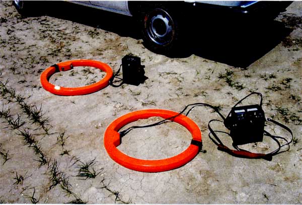
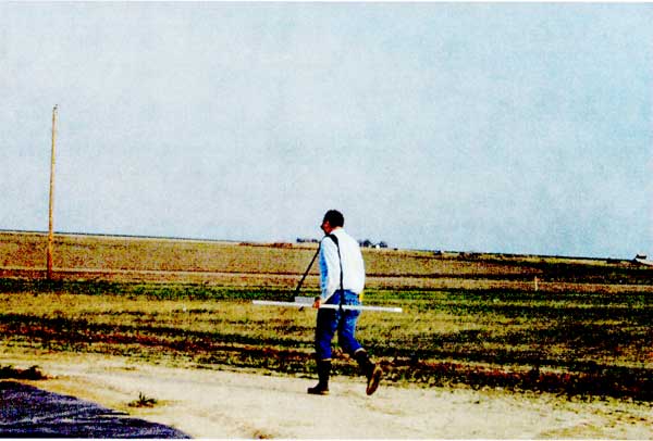
Figure 3--Geophex GEM2.
For an EM34 survey, we used three intercoll spacings--10 m, 20 m, and 40 m--as designed by Geonics, Ltd., to give variable depths of investigation. Two configurations of coils with each coil separation were used in the survey: vertical coil configuration with horizontal dipoles (HD), and horizontal coil configuration with vertical dipoles (VD). HD is the most sensitive to near surface materials and the response decreases with depth. VD is most responsive to materials located at a depth of approximately 0.4 s (s = inter-coil spacing). However, materials at a depth of 1.5 s also contribute. In the vertical dipole (horizontal coplanar) mode the EM34 is very sensitive to vertical geological anomalies and is widely used for groundwater exploration in fractured, faulted, and weathered bedrock zones. Thus, the depth of exploration is mainly a function of coil separation and orientation. The EM34 has separate coils connected by a cable that can be 10, 20, or 40 m long. Based on a homogeneous half-space assumption, the effective depths of investigation for a coil separation of 10 m with a frequency of 6.4 kHz could be 7.5 m (HD) and 15 m (VD). For coil separation of 20 m with a frequency of 1.6 kHz, investigation depths could be 15 m (HD) and 30 m (VD). For coil separation of 40 m with a frequency of 0.4 kHz, investigation depths could be 45 m (HD) and 60 m (VD) (Geonics, 1990).
Compared with the EM34, the GEM2 instrument was found to be faster and easier to operate. The GEM2 is a portable, digital, broadband electromagnetic sensor. Multifrequency data are acquired simultaneously with a maximum sampling rate of 30 Hz when the instrument operator walks along a survey line. Three frequencies were chosen for this project: 2430 Hz, 7290 Hz, and 18270 Hz. For each frequency, both in-phase and quadrature components of induced EM field in ppm (parts per million relative to the primary field) were recorded. The measured in-phase and/or quadrature responses can be used to calculate apparent conductivity based on a homogeneous half-space assumption (Won et al., 1996 and 1997). Apparent conductivity is a parameter that, in general, is related to targeted electrical properties and has units of conductivity. Apparent conductivity is a method of normalization of the EM data; it makes data analysis and interpretation easier for both geophysicists and other scientists. If the earth were truly homogeneous, the apparent conductivity would be the same at all frequencies and equal the true earth conductivity data (Huang and Won, 2001). In the real world, conductivity measurements are "bulk" or apparent conductivity. We will omit a word "apparent" in the later discussion and figures.
Quadrature data are proportional to the ground conductivity in the low to middle induction numbers, but are inversely proportional to the conductivity at middle to high induction numbers. Thus, it may occur that a moderate conductor produces a strong quadrature anomaly whereas a good conductor produces a weak anomaly or no anomaly, in which case in-phase data have to be used to further analyze the data (Huang and Won, 2001). Anomalies shown on conductivity maps should also be evident on in-phase and/or quadrature data. Investigation depth is dependent on the instrument frequency used in the survey. There is no exact relation between instrument frequency and the investigation depth.
In April 1999, a few days before the facility began operation, we conducted the first EM survey. We surveyed every 10 m along fourteen lines for a 10-m coil separation, every 10 m along twelve lines for a 20-m coil separation, and every 20 m along twelve lines for a 40-m coil separation. At each coil separation, data for both horizontal and vertical dipoles were acquired. Figures 4a-4f present the EM34 survey results in a 2-D imaging format. Crosses indicate the data location. Figures 4a-4f are ordered in terms of mapping layers from shallowest to deepest.
Figure 4--Hog lagoon, Meade County, Kansas. EM34 survey, conductivity (mS/m), April 1999.
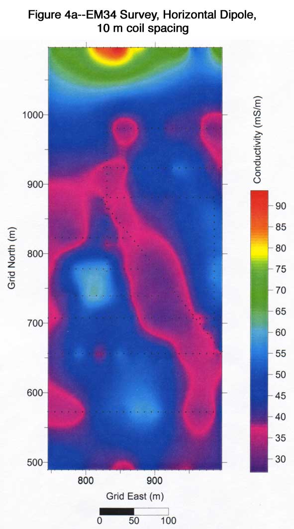
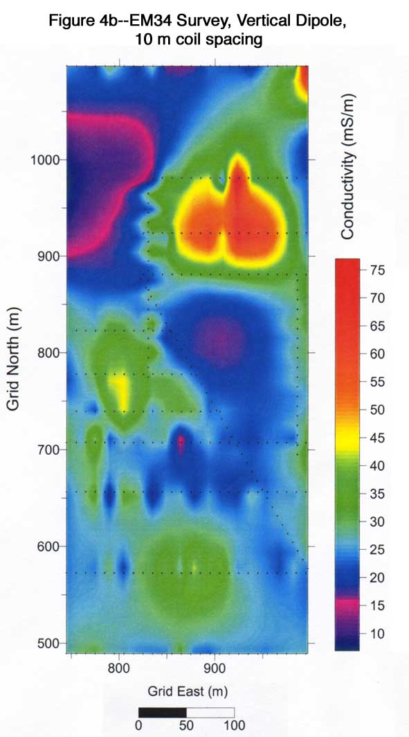
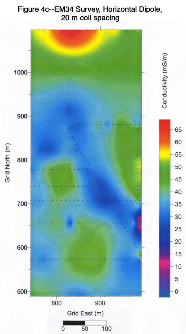
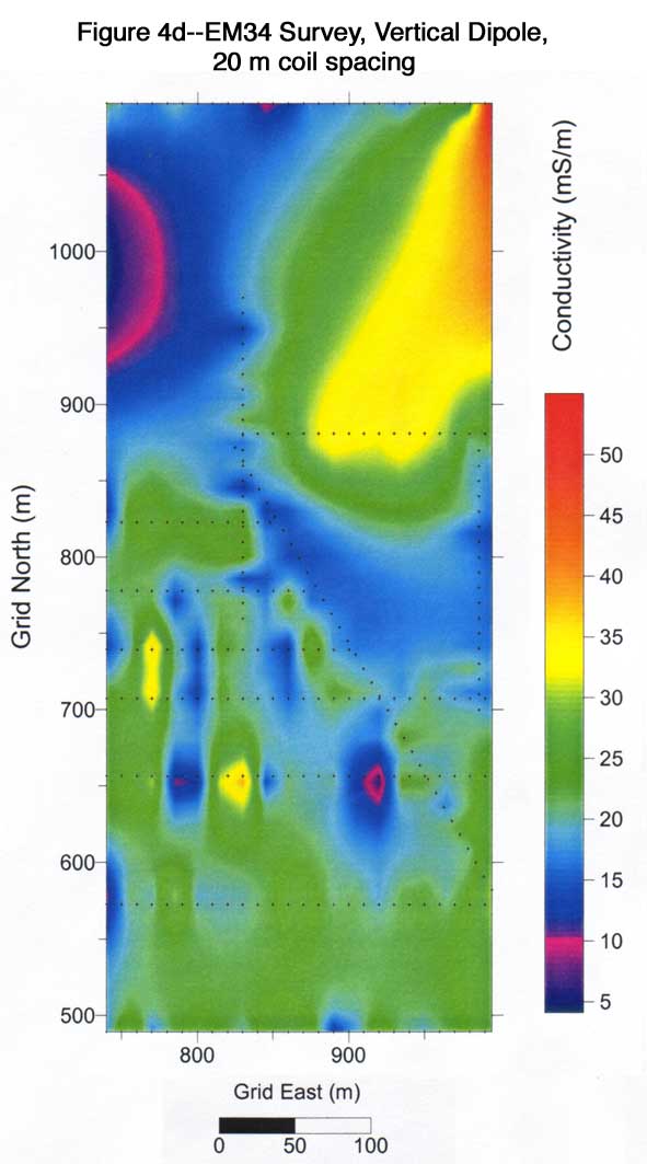
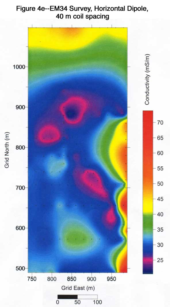
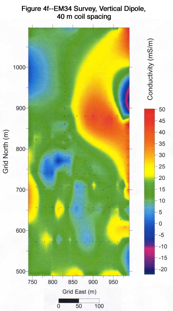
Based on a homogeneous half-space assumption, effective depths of investigation for a coil separation of 10 m could be 7.5 m for a horizontal dipole (Figure 4a) and 15 m for a vertical dipole (Figure 4b). Effective depths of investigation for a coil separation of 20 m could be 15 m for a horizontal dipole (Figure 4c) and 30 m for a vertical dipole (Figure 4d). Effective depths of investigation for a coil separation of 40 m could be 40 m for a horizontal dipole (Figure 4e) and 60 m for a vertical dipole (Figure 4f). General trends can be observed in Figure 4. First, bulk conductivities in the survey area are reduced with depth. An average bulk conductivity changes from 50-60 mS/m at a near-surface layer to 35-45 mS/m in a middle layer and then to 20-30 mS/m in a deeper layer. Second, a relatively low conductivity stripe along the northwest-southeast line is clearly shown on the horizontal dipole results (Figures 4a, 4c, and 4f). This low conductivity stripe can also be identified on the map of the vertical dipole of a 40-m separation. A conductivity high at location (890, 570) is shown on all Figure 4a-4f. Another conductivity high at location (925, 890) in Figure 4f (40-m coil separation) is caused by hog barns that are made of sheet metal. This high is also shown in a vertical dipole of 10-m and 20-m coil separations (Figure 4b and 4d).
It took one and a half days with two persons to acquire this EM34 survey after the grid was laid out.
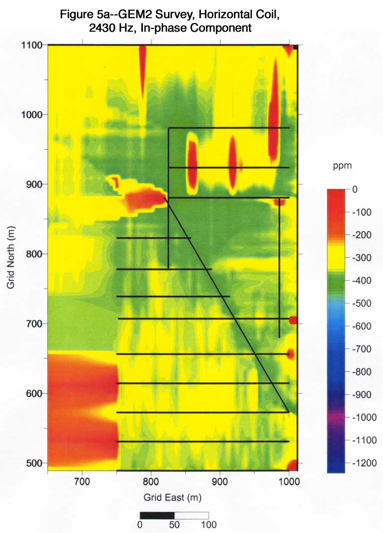
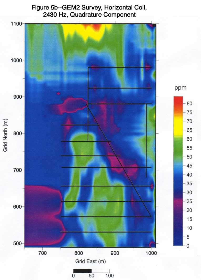
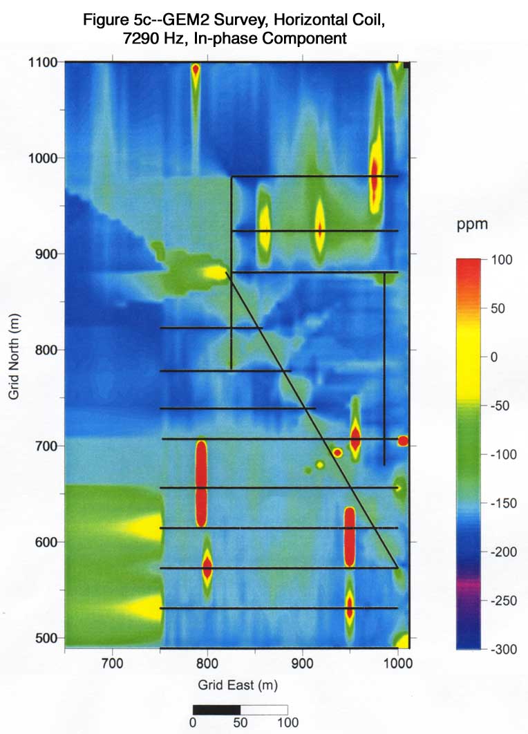
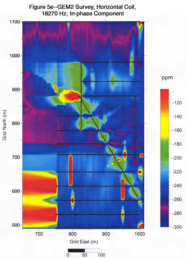
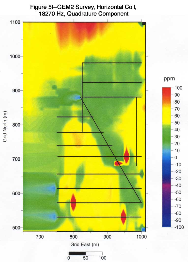
GEM2 data were acquired along seventeen lines with three frequencies: 2430 Hz, 7290 Hz, and 18270 Hz. Figures 5a-5f show the survey results of the in-phase and quadrature components for these three frequencies. The in-phase data (Figures 5a, 5c, and 5e) are much noisier than the quadrature data (Figures 5b, 5d, and 5f) because in-phase measurements are more sensitive to height of instrument than quadrature measurements when an operator was walking along lines. The line between hog barns (y = 924) shows several underground pipe lines, especially on the in-phase data (Figures 5a, 5c, and 5e).
Figure 5--Hog lagoon, Meade County, Kansas. GEM2 survey (ppm), April 1999.
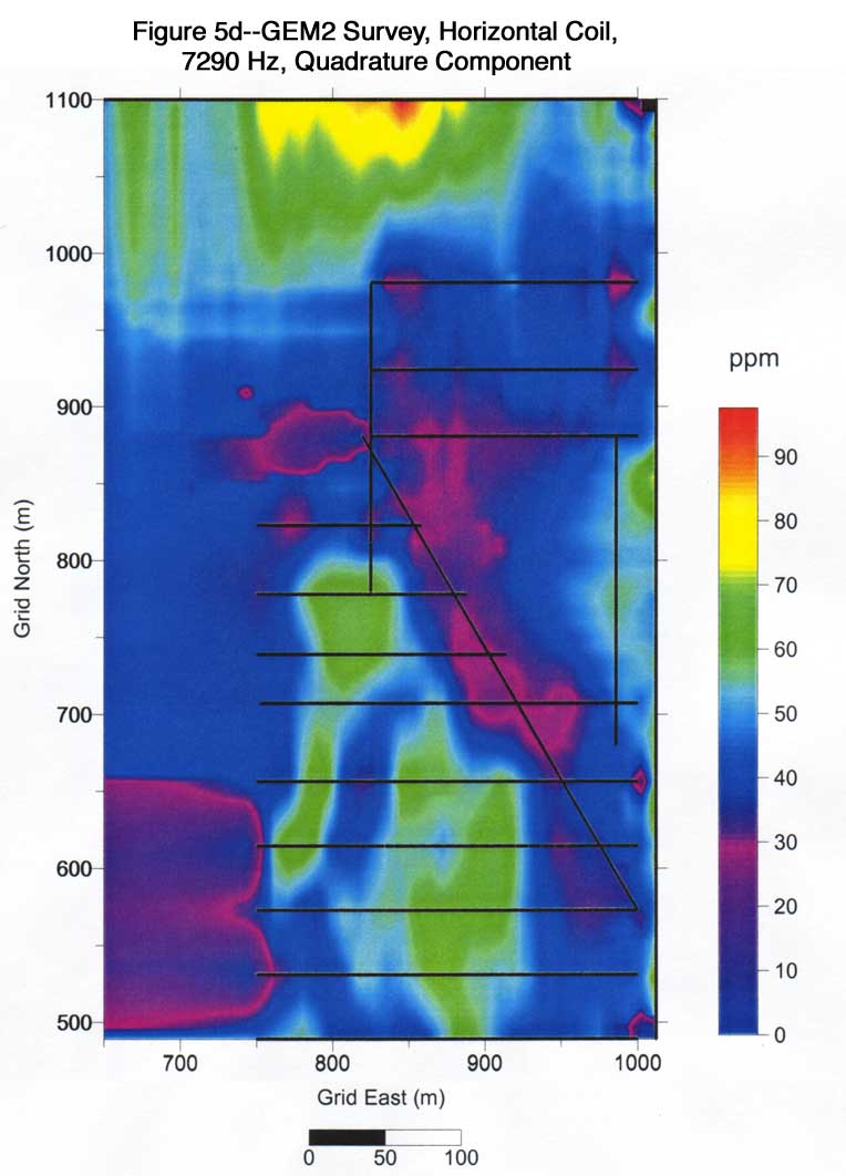
We now focus our attention on the quadrature data when comparing it with EM34 results. We are not able to compare the absolute value of conductivity for both instruments because the formulas and assumptions used in calculation of conductivity for these two instruments are different. We are more interested in relative changes and the possible similarity in terms of investigation depth.
In Figure 5b, a relative low conductivity stripe along the northwest-southeast line and conductivity high at location (890, 570) still exist. When comparing Figures 5b and 5d (2430 Hz and 7290 Hz quadrature component of GEM2) with Figure 4a (horizontal dipole 10-m coil separation of EM34), the overall pattern of both maps is similar. This pattern can also be seen in Figure 4c (horizontal dipole 20-m coil separation of EM34). This comparison gives us some idea about the investigation depth of the GEM2 instrument at this specific site. At a frequency of around 2430 Hz, the quadrature component data of a GEM2 could provide an investigation depth of 10 m to 15 m. A map of the 18270 Hz quadrature component of GEM2 (Figure 5f) shows EM properties at much shallower depth. For this reason Figure 5f cannot be compared with any maps of EM34 results.
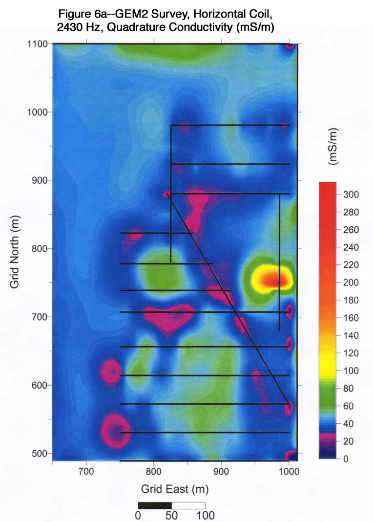
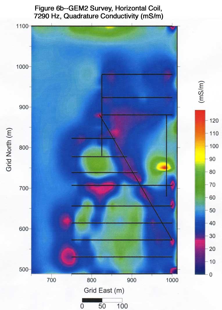
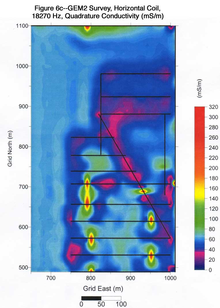
Figures 6a-6c show conductivity maps for the three frequencies. They were calculated from the GEM2 quadrature components. The patterns of the conductivity high and low indicated in the previous paragraph are also evident on these maps.
It only took one person three hours to acquire this GEM2 survey after the grid was laid out.
Figure 6--Hog lagoon, Meade County, Kansas. GEM2 survey conductivity (mS/m), April 1999.
In April 2000, after the facility operation had been in operation almost a year, we conducted the second EM survey at this site. First we used an EM34 to survey two lines. The results were compared with relevant results obtained in 1999. The results of line 656 (an east-west line) are shown in Figures 7a-7b. For horizontal dipole results, average values of conductivity for 10-m and 20-m coil separations are almost the same for both years. For vertical dipole and 10-m and 20-m coil separation results, average values of conductivity are 25 mS/m in the 1999 survey and 30 mS/m in the 2000 survey. A 40-m eastward shift (toward the lagoon) occurred on the vertical dipole and 20-m coil separation results. This shift is obviously not related to the hog lagoon.
Figure 7a--EM34 survey, 10-m coil, east-west profiles on line 656.
Figure 7b--EM34 survey, 20-m coil, east-west profiles on line 656.
Results of the line on the west lagoon wall (a northwest-southeast line) are shown in Figures 7c-7d. The horizontal dipole results for 10-m and 20-m coil separations are almost identical for both years. The vertical dipole and I 0-m separation results for both years are also the same. For vertical dipole and 20-m coil separation results, the average value of conductivity changes from 20 mS/m to 25 mS/m during the one-year period. Two single point highs at locations 230 and 270 may be due to reading or coil positioning errors. They did not change the trend of conductivity along the line.
Figure 7c--EM34 survey, 10-m coil, lagoon-wall profiles.
Figure 7d--EM34 survey, 20-m coil, lagoon-wall profiles6.
Based on these results, we conclude that after one year of operation no conductivity anomalies appeared in the depth range of investigation (20 m to 30 in).
GEM2 data were acquired along eighteen lines with three frequencies: 2430 Hz, 7290 Hz, and 18270 Hz. Figures 8a-8f show the survey results of the in-phase and quadrature components for the three frequencies. The in-phase data (Figures 8a, 8c, and 8e) are little noisier than the quadrature data (Figures 8b, 8d, and 8f), as expected.
Figure 8--Hog lagoon, Meade County, Kansas. GEM2 survey (ppm), April 2000.
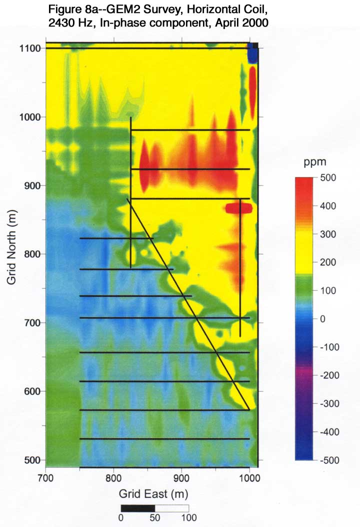
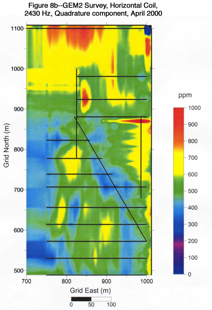
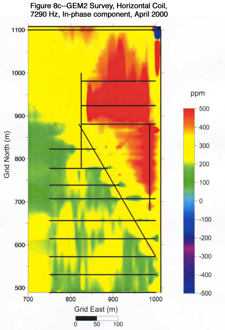
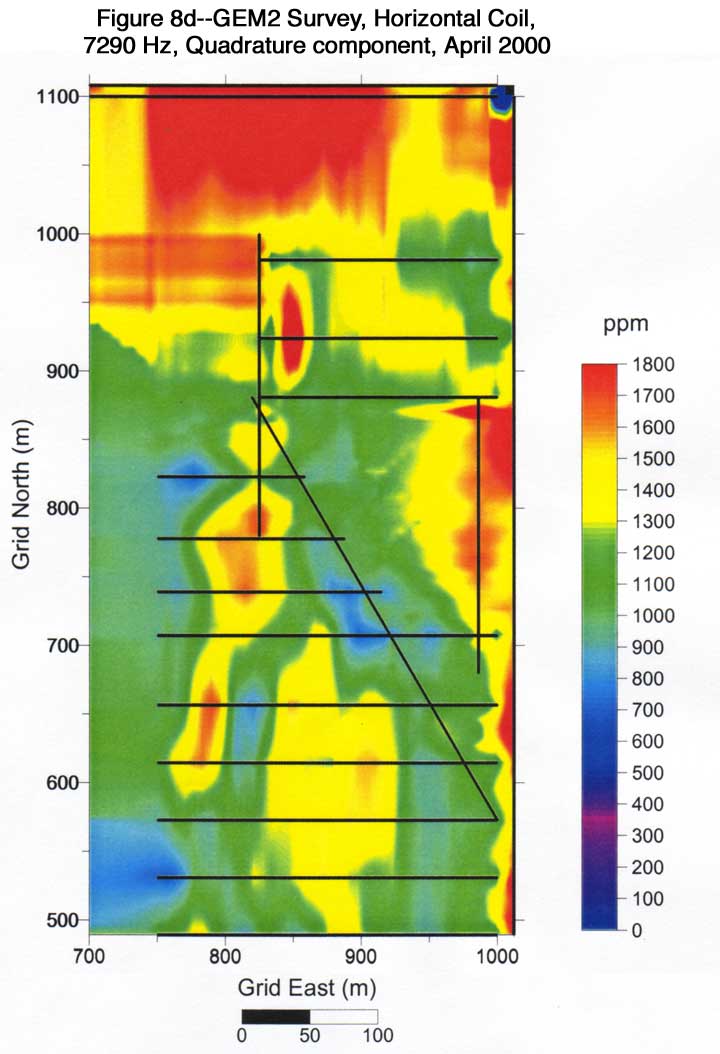
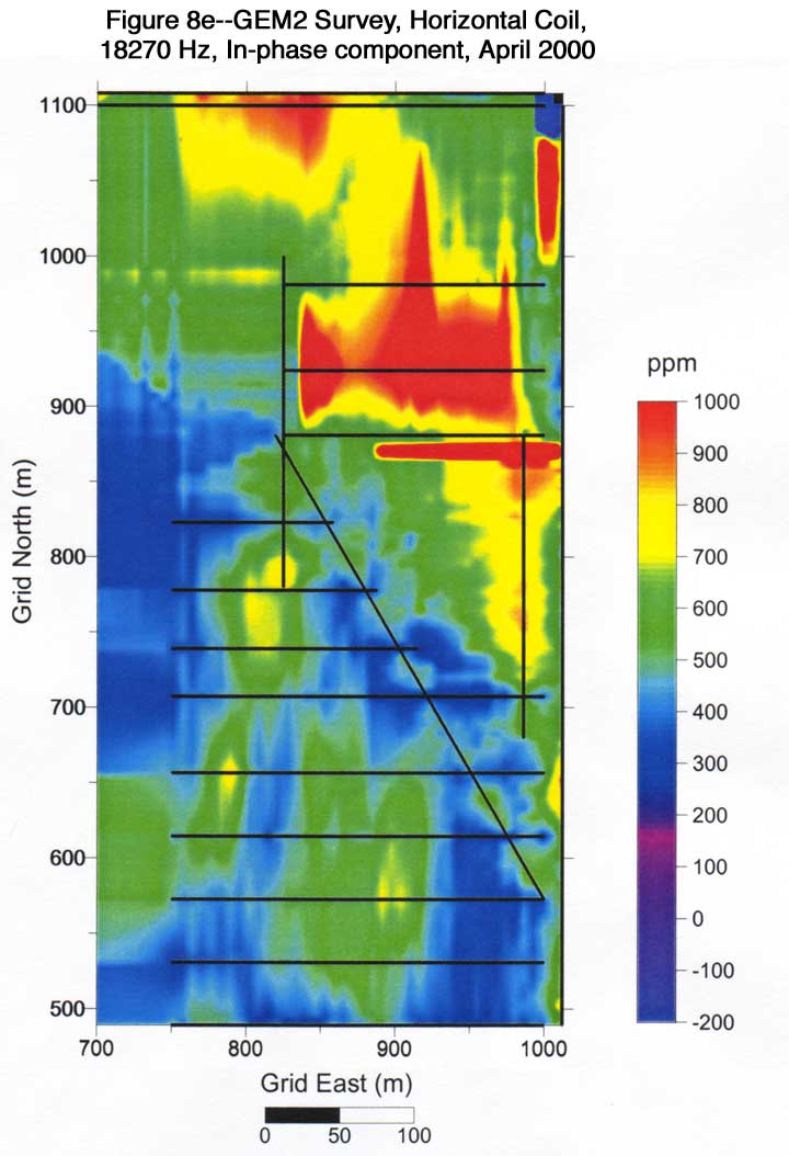
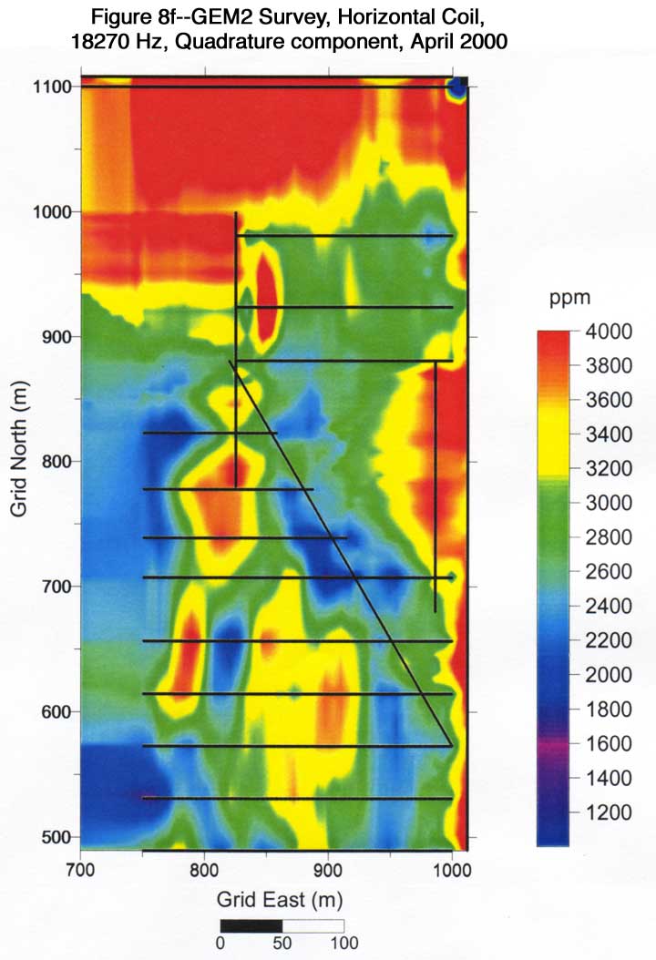
Quadrature results show the same trends and patterns that are shown on the relevant 1999 results. No dramatic changes can be identified on these maps (Figure 8) when comparing them with Figure 5. The presence of the metal hog barns affected all in-phase data.
Conductivity calculated from results in Figure 8 are shown in Figure 9a-9c. No dramatic changes can be identified on these maps.
Figure 9--Hog lagoon, Meade County, Kansas. GEM2 survey conductivity (mS/m), April 2000.
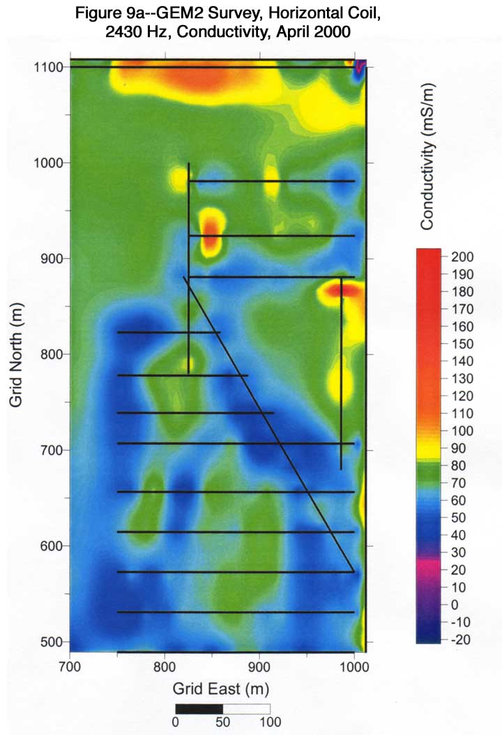
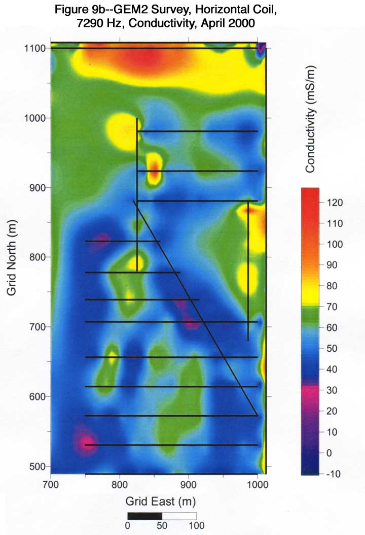
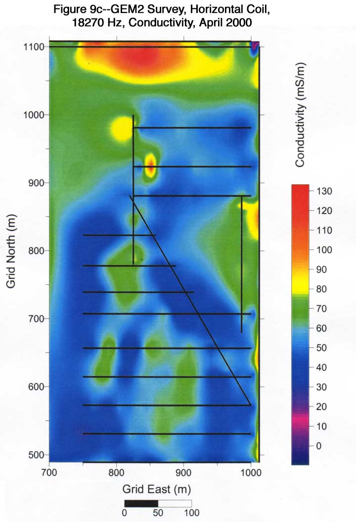
One anomaly (relative high) shown on Figures 8 and 9 at location (980, 870) was caused by a trash can, which we believe was installed after the 1999 survey. The line between hog barns (y = 924) revealed several underground metal pipes (Figure 8).
In March 2001, only GEM2 data were acquired along eighteen lines with three frequencies: 2430 Hz, 7290 Hz, and 18270 Hz. Figures 10a-10f show the survey results of the in-phase and quadrature components for three frequencies. For an easy comparison, the color scales of Figure 8 (year 2000 results) and Figure 10 are the same. Except for background reading changes, overall trends of both sets of maps remain similar. The background readings could be affected by an instrument calibration; the method to calibrate the GEM2 was changed after the 2000 survey. Again, we are more interested in relative changes in each year's survey and pattern changes in comparison to the previous year's results.
Figure 10--Hog lagoon, Meade County, Kansas. GEM2 survey (ppm), March 2001.
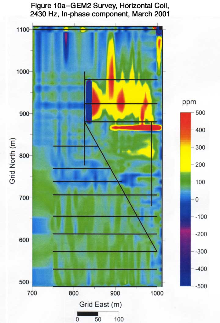
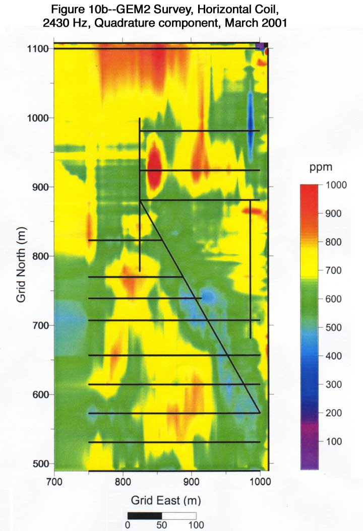
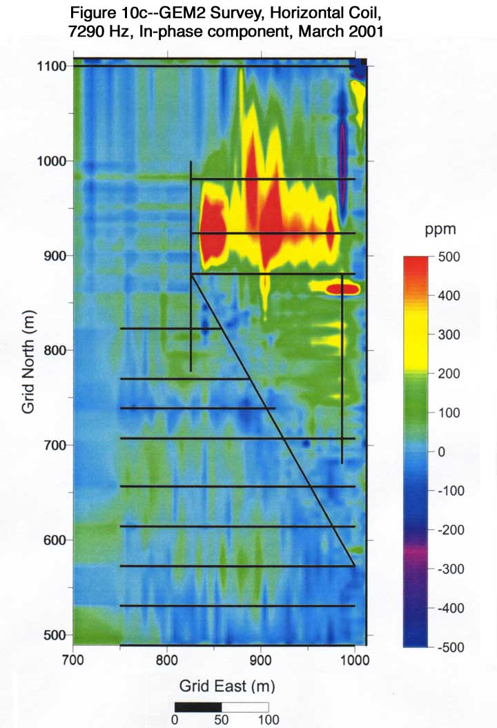
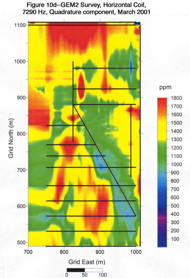
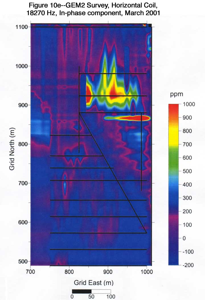
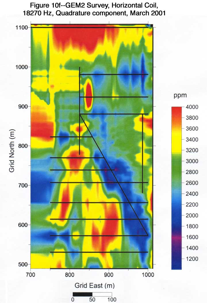
Three lines that immediately surround the lagoon gave the same results for both 2000 and 2001 in the 2430 Hz quadrature maps (Figure 8b and 10b). This indicates that no anomalous changes (several times higher than background readings) in electromagnetic readings were observed at a depth of 10 m to 15 m after a one-year period of time. The depth estimate is based on the comparison of 1999 results between the EM34 and the GEM2. After comparing 7290 Hz and 18270 Hz results for years 2000 and 2001 (Figure 8 and Figure 10), we also conclude that no dramatic changes in electromagnetic readings could be observed in the near-surface (< 10 in) during the same period of time.
Based on results of electromagnetic surveys acquired by EM34 and GEM2 instruments over a two-year period in a hog confinement facility in western Kansas, we did not find anomalous changes from the surface to a depth of 10 m to 15 m. Anomalous changes are defined as instrument readings that are significantly higher than the background readings.
GEM2 results indicate that a potential investigation depth could be up to 15 m for a frequency of 2430 Hz at this specific site after comparison with EM34 results. A GEM2 instrument can run at frequencies as low as 300 Hz, so it is possible to investigate materials up to 20 m deep. The labor requirement ratio between the EM34 and the GEM2 is more than 6. Data transfer and processing is also much easier for a GEM2 than for an EM34.
The most important advantage of an EM34 is its investigation depth. Thus, the best scenario will be to use a GEM2 for a 3-D survey (over an area) and to use an EM34 to survey several 2-D lines to calibrate the investigation depth.
We greatly appreciate advice from and discussion with Prof. Jay Ham from Kansas State University. We thank the Kansas Department of Health and Environment for lending the GM34 used in 1999 and 2000 surveys and Geophex, Ltd., for lending us the GEM2 used in the 1999 survey. We thank the farm owner, Duane Freuchting, for access to his property while performing the EM surveys. We thank Darrell Hill and John Lee of Opportunity Feedas, Inc. for their permission to do EM surveys on their property. We also thank Mary Brohammer for her effort in preparation of this report and Sihao Xia for his assistance in data acquisition.
Brune, D.E., and Doolittle, J., 1990, Locating lagoon seepage with radar and electromagnetic surveying: Environmental Geology and Water Science, 12, 195-207.
Geonics, Inc., 1990, EM-34 Users Manual, 234 pp.
Ham, J., and Desutter, T.M., 1998, Seepage losses from swine-waste lagoons: A water balance study; in Evaluation of lagoons for Containment of animal Waste: Kansas State University, K-State Research and Extension, Manhattan, KS.
Huang, H, and Won, I.J., 2001, Conductivity and susceptibility mapping using broadband electromagnetic sensors: Proceedings of the Symposium on the Application of Geophysics to Engineering and Environmental Problems (SAGEEP 2001), March 4-7, 2001, Denver, CO.
Huffman, R.L., and Westerman, P.W., 1995, Electromagnetic terrain conductivity survey methods for detection seepage plumes from animal waste lagoon: Proceedings of the Symposium on the Application of Geophysics to Engineering and Environmental Problems (SAGEEP 1995), April 23-26, 1995, Orlando, FL. 797-801.
Larson, T.H., Krapac, I.G., Dey, W.S., and Suchomski, C.J., 1997, Electromagnetic terrain conductivity surveys used to screen swine confinement facilities for groundwater contamination: Proceedings of the Symposium on the Application of Geophysics to Engineering and Environmental Problems (SAGEEP 1997), March 23-26, 1997, Reno, Nevada, 271-279.
Parker, D.B., Schulte, D.D., Eisenhauer, D.E., and Nienaber, J.A., 1994, Seepage from animal waste lagoon and storage ponds-regulatory and research review, in D.E. Storm and K.G. Casey (ed.), Proceedings of Great Plains animal waste conference on confined animal production and water quality. Denver, CO, October 19-21: Great Plans Agriculture Council, 87-98.
Won, I.J., 1980, A wideband electromagnetic exploration method--Some theoretical and experimental results: Geophysics, 45, 928-940.
Won, I.J., Keiswetter, D., Hanson, D., Novikova, E., and Hall, T., 1997, GEM-3: A Monostatic Broadband Electromagnetic Induction Sensor: Journal of Environmental and Engineering Geophysics, 2(1), 53-64.
Won, I.J., Keiswetter, D.A., Fields, G.R.A., and Sutton. L.C., 1996, GEM-2: A new multifrequency electromagnetic sensor: Journal of Environmental and Engineering Geophysics, 1(2), 129-137.
Kansas Geological Survey, Geophysics
Placed online Sept. 20, 2007, original report dated April 2001
Comments to webadmin@kgs.ku.edu
The URL for this page is http://www.kgs.ku.edu/Geophysics/OFR/2001/07/index.html