|
|
|
|
March 18, 2004, Site Visit--Start of Second Monitoring Survey |
|
|
|||
Incorporating all currently available well data, engineers project CO2 breakthrough in Colliver 12 as early as April 1, significantly ahead of preliminary schedules. Predictions of premature breakthrough at this oil-producing well have been revised based on new models that incorporate well-head data acquired during water-injection tests run just months before commencing the CO2 flood. These newer models suggest movement along the CO2 front is being influenced by high-permeability "fingers." These high-perm zones influence connectivity between Colliver 12, 14, and CO2 I1 and are likely quite thin (on the order of a seismic wavelength). It is anticipated from seismic-waveform models produced from pressure and phase relationships that as the CO2 front passes the amplitude of the reflectivity of L-KC, the C-zone reflector should change sufficiently to allow easy tracking of the CO2 plume from comparisons of images from the first two 3-D seismic surveys.
| Click on any image to view a larger version | |
|---|---|
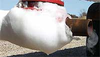
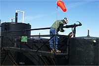
| Figure 1--Map of well locations. | Figure 2--Ice/vapor around CO2 tank vent hole. |
 |
 |
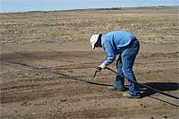
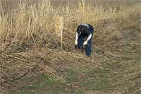
After deliberation among geologists, engineers, and geophysicists, the optimum second snapshot of the CO2 flood-monitoring survey (third 3-D survey; one baseline and two monitoring) needed to begin around March 15 (Figure 3). Based on previous experience, this third 3-D survey is expected to take about 10 days to complete. Geophones were left frozen in place after the January 2004 survey and will be used for this survey without disturbing them (Figure 4). Considering the effort taken between surveys to reoccupy identical stations and plant geophones well into competent soil, it is unlikely that leaving the receivers in place will result in distinguishable changes in survey-to-survey consistency. However, this difference will be studied and if significant improvement in waveform consistency is observed, receivers will be left in the ground where possible. Tillage of farm fields will not permit phones to remain planted in some areas of the site.
| Click on any image to view a larger version | |
|---|---|
| Figure 3--Installing cable protector across road. | Figure 4--Connecting geophones still in place after January 2004 survey to cable laid down for March 2004 survey. |
 |
 |
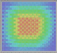
Progress processing the first two 3-D surveys (baseline during November 2003 and first monitor during January 2004) continues steadily and is expected to produce the first 3-D images around April 1st. Extra time is being spent at this stage to ensure the data processing is optimum for not only the baseline but also the dozen time-lapse surveys to follow. Design of the receiver and shot grid was based on azimuth, offset, bin squareness, fold distribution, and equipment. Using the actual shot and receiver locations occupied, it is possible to improve slightly some of the grid characteristics. In particular, the fold distribution can be improved at the expense of centralization of midpoints within the bins. By rotating the grid slightly (Figure 6), the fold uniformity improves by almost 20% with only minor increase in mid-point scatter within the bins as evidenced by the spider plots showing azimuthality and midpoint location (Figures 7 and 8).
| Click on any image to view a larger version | |
|---|---|
| Figure 5--Fold map of grid (red-24 fold; yellow-20 fold). |
Figure 6--Grid rotated 112°. |
 |
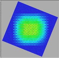 |
Rotating the grid 112° (Figure 7) retains the squareness of the 10m x 10m bins and dramatically improves the fold distribution. With every compromise comes a negative and for this improvement in fold distribution midpoint scatter within the bins increases. This scatter is clearly evident in the spider diagram (Figure 8). Even though this increased scatter in midpoint centrality is not an improvement, its effect on the overall detectability of the CO2 front should be negligible and therefore has no impact on the objectives of this research program.
| Click on any image to view a larger version | |
|---|---|
| Figure 7--Midpoints and associated rotation. | Figure 8--Spider diagram; midpoint azimuth. |
 |
 |
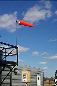
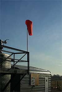
With temperatures in the 60s, ground surface dry, and winds less than 15 mph, background noise levels and site access conditions are as close to ideal for this part of the world as possible for seismic-data acquisition. When the wind exceeds 15 mph, the data quality drops sufficiently that acquisition is halted (Figure 9). Generally, during the afternoons wind velocities exceed acceptable levels for recording. To counter these unacceptable noise levels, data acquisition begins around 3:00 am and continues until wind levels exceed preset thresholds, usually occurring around 12:30 pm to 1:00 pm (Figures 9 and 10). The requirement for low wind noise is significantly more important for 4-D (time-lapse) than for standard 3-D. For 4-D to be effective, detectable changes in reflection signatures must primarily be related to changes in reservoir flood properties and not due to changes in noise levels or ground conditions.
| Click on any image to view a larger version | |
|---|---|
| Figure 9--Wind gusting at 30 mph in afternoons. | Figure 10--No wind, night and mornings. |
 |
 |
Wind noise began to become a noticeable problem when gusts exceeded 15 mph. Shot records from the end of the first day show the adverse affects of winds gusting to around 20 mph around 1:00 pm (Figure 11). Reacquiring noisy data from day 1 just 14 hours later on day 2 when winds were calm resulted in a noticeable improvement in the signal-to-noise ratio (Figure 12). A great deal of on-site effort goes into identifying shot records possessing unacceptable noise levels and reacquiring those stations when conditions are more conducive to the highest quality data possible.
| Click on any image to view a larger version |
|---|
| Figure 11--Correlated single sweep from station 13049 with 20 mph gusty winds. |
 |
| Figure 12--Correlated single sweep from station 13049 with no wind. |
 |
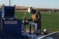
With a little over 400,000 gallons of CO2 already injected into the ground, operators and engineers are expecting breakthrough soon. The volume of fluid injected (Figure 13) and recovered (Figure 14) are both monitored very carefully, and recovery of CO2-enhanced oil is anticipated during the week of March 21.
| Click on any image to view a larger version | |
|---|---|
| Figure 13--Kevin Axelson monitoring injected CO2. | Figure 14--Kevin measures oil level in tank storing oil recovered from Colliver 12 and 13. |
 |
 |
|
Kansas Geological Survey, 4-D Seismic Monitoring of CO2 Injection Project Placed online March 19, 2004 Comments to webadmin@kgs.ku.edu The URL is HTTP://www.kgs.ku.edu/Geophysics/4Dseismic/Reports/Mar18_2004/index.html |