Goals
- Reservoir Management - Schaben Field
- study the effect on well productivities
- stimulation
- well pump rates
- infill drilling program - well placement
Volumetric Study
Prior to the start of simulation, on a grid-by-grid basis, determine
if reservoir parameters (effective porosity and net pay thickness - water
saturation) support historical production.
Determine Grid Cell & Layer Requirements
Establish grid pattern that properly defines the reservoir by using any
mapping or gridding software (Geographix used to generate the grids for
this study)
- Size Of Grid Cells In X & Y Direction
- numerical dispersion reduced - 4 to 5 grid cells between wells
- grid sizes of 220 ft by 220 ft - 5 grid blocks between wells
Determination of Layers for Simulation
- reservoir heterogeneity
- schaben field is a dual porosity - dual permeability system
- oil column migrated across multiple zones
- most cores contain vertical fractures
- mini-permeameter results - high & low permeability layers
- production history - initial water free production followed by rapid
onset of water production
- current reservoir pressure near original reservoir pressure - suggests
strong recharge by aquifer
- multiple completions in isolated reservoirs
- segregate openhole & casedhole completions by layer
Number & size of grid cells in Z direction
Simulation designed as two layer model - a reservoir layer with an underlying
aquifer layer. Z-dimension equals pay thickness (top of the reservoir to
the OWC, average depth of OWC = -2145 ft subsea)
Layer 1 - Reservoir (gross/net pay thicknesses assumed to be equal)
- difficult to distinguish between productive and non-productive zones
- porosity and permeability averaged over pay thickness
Layer 2 - aquifer provides recharge to reservoir layer (aquifer thickness
in Schaben Field approximately 100 feet)
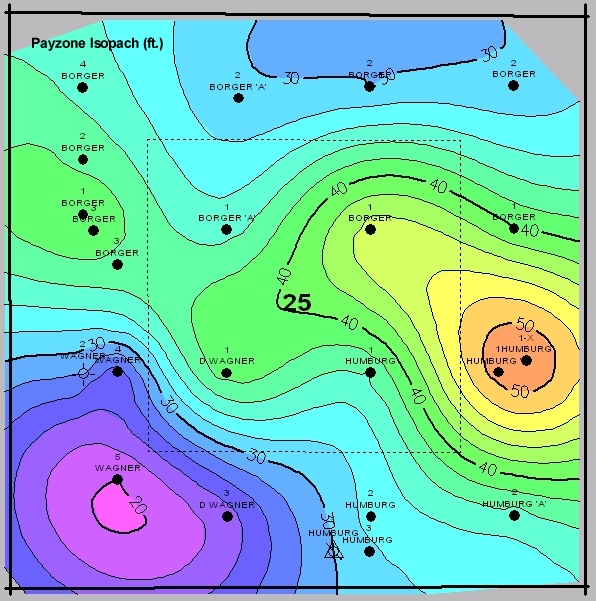
Reservoir parameters
- Pay thickness - grid dimension in z direction
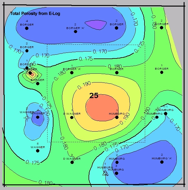
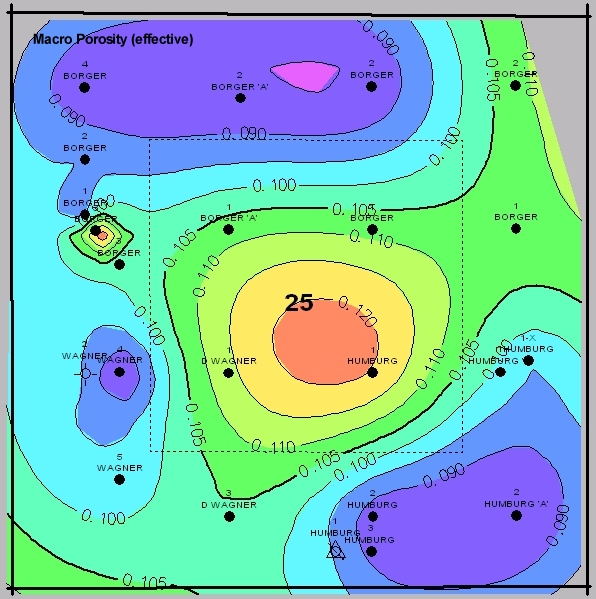
- Porosity
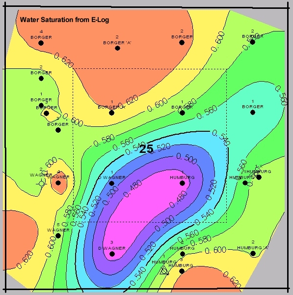
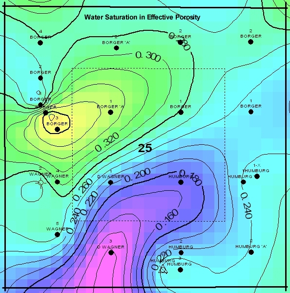
- fluid saturations
- dichotomy - Sw from petrophysical logs & production history
- average Sw - 65 to 75%.
- production history - high OWR in early years followed by water break
through
- thus all of Sw is not mobile
- effective saturation calculations on grid cell basis
- OOIP = (1-Sw) * grid volume * total porosity
- effective pore volume = grid volume * effective porosity
- effective So = OOIP / (effective pore volume)
- effective So - normalized <= 75% - relative permeability curves
indicate Swi = 25%
- effective Sw = 1- (effective So) (water saturation in effective porosity)
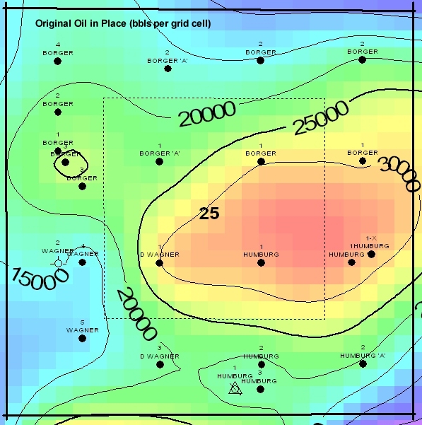
- Map of OOIP on a grid cell basis - effective
porosity * effective So * grid volume
- Map of cumulative production
- Available production history - 33 years lease production history &
well productivity tests.
- Calculate well production - annual productivity tests - distribute
lease production to wells. Bo (=1.04) - surface volume to reservoir volume.
- Schaben Field - uniform 40 acre spacing with 36 grid cells per acre.
- Cumulative production per well divided by 36 (grid cells) to allocate
production over drainage area to generate cumulative production per grid
cell map.
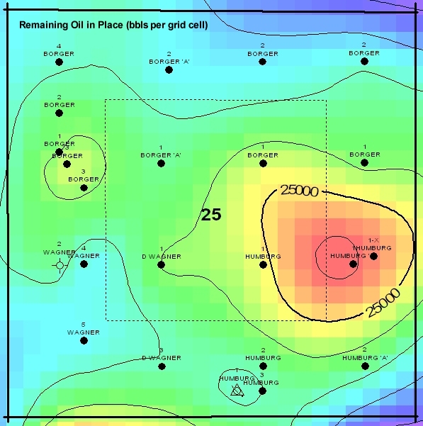
- Map of ROIP per grid cell
- ROIP = OOIP – cumulative production
- remaining So = ROIP / effective pore volume
- remaining So thickness = remaining So * pay thickness
- Soir = 25% (assumption)
- residual mobile So = remaining So - Soir - So => 0 - reservoir parameters
consistent with production history
- Sor * t = residual mobile So * pay thickness - buried treasure map
- areas with significant production potential
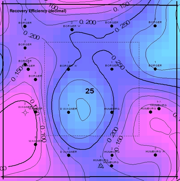
- Map of Recovery Factor - on a grid cell basis
– cumulative production / OOIP
e-mail : webadmin@kgs.ukans.edu
Updated January 1999
The URL for this page is http://www.kgs.ukans.edu/General/Tutorial/Boast3/exergoals.html