HELP: Quantitative Analysis Equations - Gas DST

NOTE: Much of this web page is taken from the lecture notes "Modern Concepts in Drillstem Testing Part 2 Quantitative Analysis"² by Hugh W. Read, Author & Instructor.

Conventional Horner Type Pressure Buildup Analysis Conditions Assumed for Analysis Procedure

For a disccussion of the theory of pressure buildup interpretaton and the derivation of the pertinent equations the reader is referred to the original now classical paper by Horner⁽¹⁾.

90% of all quantitative Drill Stem Test analysis is based on Horner's method of analysis which assumes the following ideal conditions:

i) Radial flow
Radial flow is flow into the well bore equally from all directions in the formation. By and large condition is met by most DST's through linear systems such as fractures, narrow channel sands etc. are obvious exceptsion which may be handled separately.

ii) a homogeneous reservoir
Homogeneity in a reservoir denotes constant characteristics throughout the length and thickness. Any values calculated from test data then becomes averages over the length and/or thickness.

iii) "steady-state" conditions of flow
"Steady-state" flow condiitions imply a rate and pressure drawdown (which is responsible for the flow) which is constant.

iv) infinite reservoir
An infinite reservoir is one in which there are no finite limits or depletion. All DST's in wildcat wells can be considered to test infinite reservoirs, except those testing very small local porosity or fracture developments which in any event deplete rapidly and are not commercial.

v) single phase flow
Single phase flow assumes that only one phase is entering the well bore. Thus for example any gas produced with oil is considered as solution gas and any liquids in a gas test are considered as condensation of gases in the pipe or immediate well bore vicinity.

Method of Construction of Horner plot - Gas Drill Stem Test

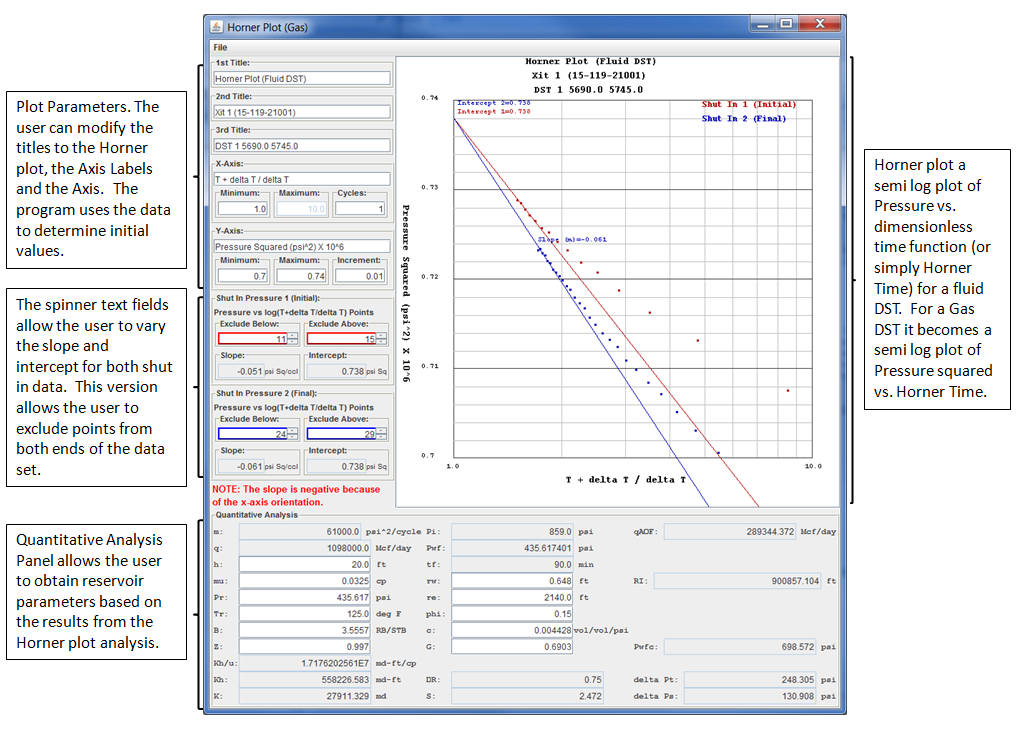
This example is from the Xit 1; DST 1 in the Upper Kearny Member from 5690.0 ft to 5745.0 ft dst-gas.las. The Gas Rates and Pressure Summary Data will be needed in performing the plot and quantitative analysis and is listed as follows,

Gas Rates Table Flow Elapsed Pressure Gas Rate Choke Period Time (psig) (Mcf/day) (in) 1 10.0 14.0 577000.0 1.0 1 20.0 24.0 817000.0 1.0 1 30.0 28.0 907000.0 1.0 2 10.0 26.0 865000.0 1.0 2 20.0 33.0 1012000.0 1.0 2 30.0 35.0 1057000.0 1.0 2 40.0 36.0 1076000.0 1.0 2 50.0 36.0 1076000.0 1.0 2 60.0 37.0 1098000.0 1.0

Pressure Summary Table Time Pressure Temperature Annotation (min) (psig) (deg F) 0.0 2748.7854 122.407204 Initial Hydrostatic 5.5 155.137894 123.1147 Open to Flow 1 36.0 496.501312 121.527901 Shut-in 1 96.0 853.742798 126.989899 End Shut-in 1 97.0 233.796402 126.3834 Open to Flow 2 156.5 435.617401 115.143501 Shut-in 2 280.0 850.436829 125.351997 End Shut-in 2 285.5 2727.0625 126.5923 Final Hydrostatic

See the paper "Recent Developments in the Interpretation and Application of DST Data" by L.F.Maier⁽³⁾. There were a number of DST papers that seem to use the Pressure squared method. Reid suggests that the linear Horner plot was sufficient. A future version of the DST Tool may allow the user to select between Pressure or Pressure squared in a Horner plot analysis.

(1) The data necessary for this plot is a set of detailed readings of pressures and times during each shut in period plus the total amount of time spent flowing the well.

(2) Arrange the data in tablular form where,

T = Cumulative flowing time (minutes)
ΔT = Times during shut in that each pressure is read (minutes)
P = Pressure read during shut in time (psig)
P² = Pressure squared (psig²)

Shut In 1 (Initial) Total Flow Time (T) = 30 minutesa Time (ΔT) (T+ΔT)/ΔT Pressure (P) Temperature Pressure squared (P2) (min) (psig) (deg F) (psig2) 0.0 --- 496.501312 121.527901 246,512.25 4.0 8.50 841.170715 125.614502 707,566.97 8.0 4.75 844.496826 126.780701 713,180.25 12.0 3.50 846.328003 126.656998 716,274.47 16.0 2.88 847.812927 126.512199 718,781.80 20.0 2.50 848.991882 126.430603 720,784.02 24.0 2.25 849.629028 126.429497 721,871.14 28.0 1.07 850.446777 126.441704 723,265.20 32.0 1.94 850.998596 126.487801 724,201.00 36.0 1.83 851.615723 126.541397 725,256.62 40.0 1.75 851.901672 126.6035 725,733.61 44.0 1.68 852.340271 126.679298 726483.48 48.0 1.63 852.739502 126.757896 727,165.51 52.0 1.57 853.130676 126.837502 727,830.80 56.0 1.54 853.542114 126.921898 728,530.53 60.0 1.50 853.742798 126.989899 728,871.99		Shut In 2 (Final) Total Flow Time (T) = 59.25 + 30 = 89.25 minutesb Time (ΔT) (T+ΔT)/ΔT Pressure (P) Temperature Pressure squared (P2) (min) (psig) (deg F) (psig2) 0.0 --- 435.617401 115.143501 189,764.78 4.0 23.31 825.081787 119.8134 680,757.01 8.0 12.16 830.118713 121.163101 689,099.21 12.0 8.44 833.033508 121.227501 693,938.98 16.0 6.68 835.235901 121.179703 697,625.86 20.0 5.46 837.006775 121.144402 700,585.74 24.0 4.72 838.476685 121.177597 703,048.71 28.0 4.19 839.725891 121.214996 705,146.47 32.0 3.79 840.914917 121.298103 707,129.63 36.0 3.48 841.682373 121.412399 708,425.22 40.0 3.23 842.520203 121.562202 709,839.95 44.0 3.03 843.182373 121.730797 710,952.51 48.0 2.86 844.06543 121.915604 712,454.16 52.0 2.72 844.552002 122.107803 713,264.70 56.0 2.59 844.938416 122.306 713,923.60 60.0 2.49 845.54541 122.5158 714,954.80 64.0 2.39 846.011902 122.712097 715,732.92 68.0 2.31 846.609009 122.936401 716,748.49 72.0 2.24 846.955078 123.124702 717,341.24 76.0 2.17 847.331421 123.330902 717,968.13 80.0 2.12 847.858093 123.534203 718,866.58 84.0 2.06 848.078918 123.712997 719,239.69 88.0 2.01 848.460205 123.904503 719,884.37 92.0 1.97 848.756104 124.090897 720,393.54 96.0 1.93 848.997009 124.264297 720,801.00 100.0 1.89 849.177612 124.4431 721,106.67 104.0 1.86 849.583923 124.618301 721,786.18 108.0 1.83 849.724426 124.773598 722,024.08 112.0 1.80 850.115723 124.930603 722,704.01 116.0 1.77 850.256226 125.089798 722,942.07 120.0 1.74 850.521973 125.233299 723,384.27 124.0 1.72 850.436829 125.351997 723,231.18
From the Pressure Summary Table (a) Shut-in 1 Time - Open to Flow 1 Time { 38.5 - 8.5 = 30.0 minutes } (b) Shut-in 2 Time - Open to Flow 2 Time + Total Flow Time from (a) { 159.0 - 99.75 + 30.0 = 89.25 minutes }

In the table note that the Shut In 1 & 2 periods were broken down into 4 minute intervals.

The Pressure Summary Table gives a summary of the DST Pressure-Temperature-Time Readings at specific points. This DST had a 30.0 minute preflow and a 59.25 minute main flow. Thus 'T' for the Shut In 1 (Initial) period = 30.0 minutes since there was a total of 30 minutes flow time prior to Shut In 1 (Initial). T for the Shut In 2 (Final) period becomes 89.25 minutes ( 30 minutes preflow + 59.25 minutes mainflow since T is the cumulative flow time prior to shut in.

The quantity (T + ΔT)/ΔT is mathematically the same as 1 + (T/&DeltaT) thus for the Shut In 2 (Final) period example the (T + ΔT)/ΔT for the first increment = (89.25+4)/4 = 23.31, which is the same as 1 + (89.25/4) = 1 + 22.31 = 23.31.

(3) The Horner plot is then constructed by plotting log₁₀[(T+ΔT)/ΔT] vs P² for each point.

Figure 2. Horner Plot for Gas DST

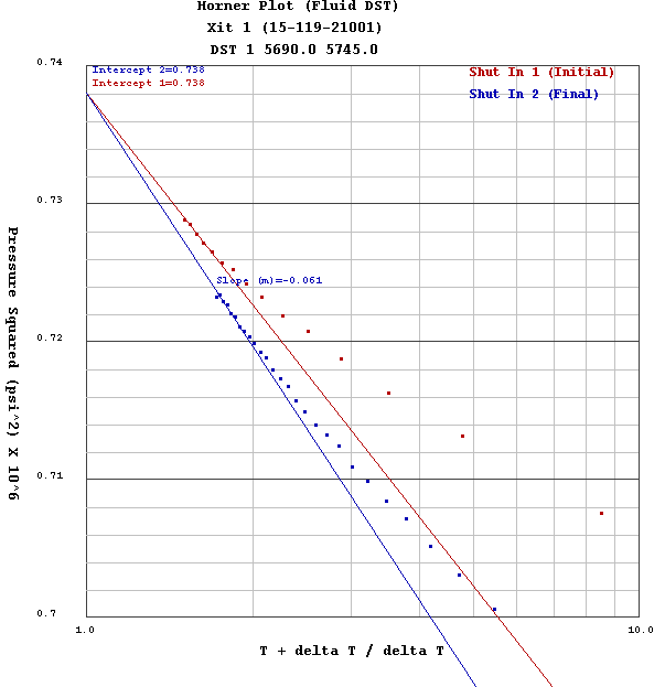
(4) In Figure 2 both Shut In Pressure-Time curves have been plotted. In order to determine the static reservoir pressure the linear portion is extrapolated to the left hand margin where the value of the time function (T + ΔT)/ΔT = 1. Since the logarithm of 1 is zero the log₁₀[(T + ΔT)/ΔT ] = 0 (or infinity) at this point. Thus we are extrapolating the Horner straight line to a 'infinite' shut in time where completely static pressure prevails. In the example here the static pressure squared ~ 738,000.0 psig² or 859.0 psig. Both Shut In intervals extrapolations yield this value. In cases where the Shut In 2 (Final) extrapolation is substantially less than the Shut In 1 (Initial) depletion is indicated. ( If the depletion factor 100.0 * Shut In [(Initial)-(Final))/(Initial) ] is greater than 4%, then the idications of depletion can be considered serious or sustantial.

(5) The final piece of information which is obtained form the Horner plot is the "slope" (m) of the striaght line segment. Numerically this is the difference between the pressure at log₁₀[(T + ΔT)/ΔT ]=0 and at log₁₀[(T + ΔT)/ΔT ]=1. where the slope is simply the change in pressure over one complete log cycle. The slope in this example using the Shut In (Final) slope m=0.061 psi²/cycle. The slope is used in the calculations to derive permeability and other reservoir parameters.

Transmissibility (K*h/μ), Permeability Thickness (K*h), Permeability (K)

The pressure build-up equation applicable to gas wells is expressed by

Po² = Pf² - m_g * log₁₀[(T+ΔT)/ΔT].

The build-up plot of Po² vs. log₁₀[(T+ΔT)/ΔT] is constructed and extrapolated to log₁₀[ (T+ΔT)/ΔT ] to zero to obtain Pf² and m_g, the slope of the line.

m_g = 1632 * q_g * μ * Z * Tf / (K * h) [psi²] / [log cycle]
q_g = flow rate [Mcf] / [day]
μ = viscosity [cp]
Z = Gas Deviation Factor ( Compressibility factor)
Tf = Formation Temperature [^oR]; ^oR = ^oF + 459.67
h = vertical thickness of continuous porosity [ft]
K = average effective permeability [md]

This states that the slope of the buildup is representative of a given fluid having physical properties μ, Z, Tf flowing at a rate q_g through a formation having physical properties K * h.

Note: the flow rate (q) is computed by using an average of the final gas rates in the gas rates table.

Transmissibility can be found my rearranging the slope as follows,

Transmissibility:	K * h / μ = 162.6 * q * B / m	[md]-[ft]/[cp]
Permeability Thickness:	K * h = ( Transmissibility ) * μ	[md]-[ft]
Permeability:	K = ( Permeability Thickness ) / h	[md]

Damage Ratio (DR), Skin factor (S), and related quantities

Damage Ratio (DR) - A numerical value used to predict the flow rate if the damage were removed. In essence the DR becomes a number which when multiplied by the flow rate which existed at the time of the test will yield the flow rate if the damage (or improvement) over the natural condition is removed. This flow rate will be the rate at the same flowing pressure drawdown which existed during the test. From the definition of DR if a zone is neither damaged nor improved then q theoretical is identical to q actual and DR = 1.

	Pi2 - Pwf2
DR =	------------------------------------------------	- 2.85
	mg * log { [ k * To / ( φ * μ * c * rw2 ) ] }

where,

Pi	= Initial static reservoir pressure	[psig]
Pwf	= Bottom Hole Flowing Pressure (FFP)	[psig]
mg	= slope from the Horner plot	[psi] / [log cycle]
K	= Permeability ( K )	[md]
To	= Flow Time	[min]
φ	= Porosity
μ	= viscosity	[cp]
c	= compressibility	[vol]/[vol]/[psi]
rw	= well bore radius	[ft]

If K, φ, μ, c and r_w are not known then the Damage Ratio can be estimated by,

	Pi2 - Pwf2
EDR =	-----------------	+ 2.65
	mg * log { To }

Skin factor (S) - A numerical quantity which attempts to describe the amount of damage or improvement. The numerical value of skin is so defined that a positive value for the skin factor indicates a damaged condition and a negative skin factor indicates improvement over the natural condition. The skin factor is zero when neither skin damage nor improvement are present i.e. no alterations to natural condition.

	-					-
	|	Pi2 - Pwf2		K * To		|
S = 1.1515 *	|	--------------	- log	------------------	+ 5.01	|
	|	mg		φ * μ * c * rw2		|
	-					-

Pi	= Initial static reservoir pressure	[psig]
Pwf	= Bottom Hole Flowing Pressure (FFP)	[psig]
mg	= slope from the Horner plot	[psi] / [log cycle]
K	= Permeability ( K )	[md]
To	= Flow Time	[min]
φ	= Porosity
μ	= viscosity	[cp]
c	= compressibility	[vol]/[vol]/[psi]
rw	= well bore radius	[ft]

If φ, μ, c and r_w are not known then the Skin factor (S) can be estimated by,

	-					-
	|	Pi2 - Pwf2				|
S = 1.1515 *	|	-----------	- log	(K * To * Pi)	+ 1.40	|
	|	mg				|
	-					-

Pressure Drop Across a Damage Zone ΔP_skin The additional pressure drop during flow caused by the presence of skin (ΔP_skin) may be calculated as follows,

ΔP_skin = - Pwf + √( Pwf² + 0.87 * S * m )

where,

S	= Skin factor
Pwf	= Bottom Hole Flowing Pressure (FFP)	[psig]
m	= slope from the Horner plot	[psi] / [log cycle]

Radius of Investigation (RI) The radius of investigation is the radial distance from the well bore which the pressure disturbance from the DST has investigated ( in other words "how far out into the zone the DST has looked").

RI = 2.6408 * √( K*To / ( φ * μ * c ) )

where,

Pi	= Initial static reservoir pressure	[psig]
K	= Permeability ( K )	[md]
To	= Flow Time	[min]
φ	= Porosity
μ	= viscosity	[cp]
c	= compressibility	[vol]/[vol]/[psi]

If φ, μ, and c are not known then the Radius of Investigation (RI) is as follows,

For Gas: RI = 0.125 * √( K * Tf * Pi )

Effects of Turbulence⁽²⁾ The skin factor and damage ratio values computed from the preceding equations do not take account of the additional pressure drop which is caused by turbulence in gas flow. The turbulence factor is not easy to determine precisely in DST's, however, an approximate empirical relationship between turbulence and permeability has been determined.

Step 1 The flowing pressure corrected for turbulence (Pwfc) is computed as follows,

		-					-				-	-
		|			0.129 * G * Tf * Z * q2		|	1		1	|	|
	Pwfc = √	|	(Pwf + 14.65)2	+	----------------------------	*	|	--	-	--	|	|
		|			K4/3 * h 2		|	rw		RI	|	|
		-					-				-	-

	Pwf	= Bottom Hole Flowing Pressure (FFP)	[psig]
	G	= Gas Specific Gravity (air = 1)
	Tf	= Formation Temperature	[oR]; oR = oF + 459.67
	Z	= Gas Deviation Factor ( Compressibility factor)
	q	= Flow Rate -	[ Mcf ] / [ Day ]
	K	= Permeability	[md]
	h	= thickness	[ft]
	rw	= well bore radius	[ft]
	RI	= Radius of Investigation	[ft]

Step 2 The value of (Pwfc) is then substituted for (Pwf) in the skin factor (S) and damage ratio (DR) equations to determine the true skin factor (S) and damage ratio (DR) to exclude the effects of turbulence.

Step 3 The pressure drop due to turbulence (ΔP_t) may also be of interest and may be calculated simply as,

ΔP_t = - Pwf + √( Pwf² + 0.87 * m_g * S )

Absolute Open Flow Capacity (qAOF) A theorectical quantity which describes the maximum flow rate of a gas zone at zero sandface pressure. It is an unattainable rate in practice but from it may be derived the flow rates at any practical flowing pressure.

Houpert equation: Pi*Pi - Pwf*Pwf = a*q + b*q*q, where

	1424 * Tf * Z
a (Laminar Flow) =	------------------	* ( ln(re/rw) - 0.75 + S )
	(K * h / μ)

	0.129 * G * Tf * Z
b (turbulence factor) =	------------------------	* ln ( (1/rw) - (1/re) )
	K4/3 * h2

Pwf = 0 by definition

	-a + √( a * a + 4 * b * Pi * Pi )
qAOF=	----------------------------------------
	2 * b

Pi	= Initial static reservoir pressure	[psig]
Pwf	= Bottom Hole Flowing Pressure (FFP)	[psig]
K	= Permeability ( K )	[md]
h	= vertical thickness of continuous porosity	[ft]
μ	= viscosity	[cp]
Z	= Gas Deviation Factor ( Compressibility factor)
Tf	= Formation Temperature	[oR]; oR = oF + 459.67
G	= Gas Specific Gravity (air = 1)
re	= drainage radius	[ft]
rw	= well bore radius	[ft]

If b = 0 then qAOF = Pi * Pi / a

References:
(1) Pressure Build-Up in Wells, by D.R. Horner, 3rd World Petroleum Congress, May 28 - June 6, 1951 , The Hague, the Netherlands http://www.onepetro.org/mslib/servlet/onepetropreview?id=WPC-4135&soc=WPC
(2) Drillstem Test Interpretation Seminar, Author & Instructor: H.W.Reid
(3) Recent Developments in the Interpretation and Application of DST Data, by L.F.Maier Journal of Petroleum Technology Volume 14, Number 11, November 1962, pgs 1213-1222 http://www.onepetro.org/mslib/servlet/onepetropreview?id=00000290