---

Start
Contents
Introduction
Climate
General Geology
Ground Water Geology
Irrigation
Water-bearing Materials
Water Table
Availability
Chemical Character
Well Records
Logs
References
Plates

Prev Page--Ground Water Geology || Next Page--Water Table

---

Hydrologic Properties of the Water-bearing Materials

The quantity of ground water that an aquifer will yield to wells depends upon the hydrologic properties of the materials in the aquifer. The principal hydrologic properties of an aquifer are its ability to transmit and to store water. The ability of an aquifer to transmit water is measured by its coefficient of transmissibility, and the ability to store water is measured by its coefficient of storage—a coefficient indicating the quantity of water that will be yielded from storage when the head is lowered.

The coefficient of transmissibility (T) of a water-bearing formation is expressed as the rate of How of water, in gallons per day, at the prevailing temperature through a vertical strip of the aquifer 1 mile wide extending the full height of the aquifer under a hydraulic gradient of 1 foot per mile. The field coefficient of permeability (P) is expressed as the rate of How of water, in gallons per day, at the prevailing temperature through each mile of the aquifer for each foot of thickness under a hydraulic gradient of 1 foot per mile. The field coefficient of permeability can be computed by dividing the coefficient of transmissibility by the aquifer thickness (m). The coefficient of storage of an aquifer may be defined as the volume of water it releases from or takes into storage per unit surface area of the aquifer per unit change in the component of head normal to that surface. Under water-table conditions the coefficient of storage is practically equal to the specific yield, which is defined as the ratio of the volume of water a saturated material will yield to gravity in proportion to its own volume.

Purpose of Aquifer Tests

The well inventory and test drilling in the Ingalls area indicated several physical factors that would affect the maximum perennial yield of wells in the Arkansas Valley. These factors are the flow of Arkansas River; the thickness, areal extent, and lithology of the alluvium; the hydraulic connection between the river channel and the alluvium; the thickness, areal extent, and lithology of the Ogallala formation; and the hydraulic connection between the alluvium and the underlying Ogallala formation.

To determine the hydraulic connection between the river and the alluvium and between the alluvium and the Ogallala formation, it was necessary to determine the hydraulic constants of transmissibility, permeability, and storage of these aquifers. In addition, it was necessary to determine the vertical permeability of the Ogallala formation, as test drilling had shown that massive silt and clay confining beds were present below the alluvium and could prevent downward percolation of water from the alluvium to the Ogallala formation. Seven aquifer tests were made to determine the hydraulic constants.

Three aquifer tests were made in the alluvium. The first test was made to determine the coefficients of transmissibility and storage. The second and third tests were made not only to determine the coefficients of transmissibility and storage, but also to determine the extent of the hydraulic connection between Arkansas River and the alluvium.

Four aquifer tests were made in the Ogallala formation. Two were recovery tests made in the upland to determine the coefficient of transmissibility. Two were made in the Ogallala formation underlying the alluvium and were designed to determine not only the transmissibility and storage coefficients, but also the vertical coefficient of permeability of the Ogallala formation and the recharge from the alluvium to the underlying Ogallala formation.

Methods

The data collected during the aquifer tests were analyzed by the methods generally referred to as the Thiem method, the Theis non equilibrium method, the Jacob modified nonequilibrium method, and the Jacob leaky-aquifer method. All these methods were used where applicable to arrive at the best interpretation of the aquifer-test data.

Thiem method

The Thiem method is a means for determining the coefficients of transmissibility and storage on the basis of the rate of discharge of a pumped well and the drawdown in each of at least two observation wells at different known distances from the pumped well. The Thiem equation (Wenzel, 1942, p. 81), expressed in terms of transmissibility instead of permeability, is r2

T = [527.7 Q log₁₀ (r₂ / r₁)] / s₁ - s₂

where T is the coefficient of transmissibility, in gpd/ft,
Q is the rate of discharge of the pumped well in gpm,
r₁ and r₂ are the respective distances of two observation wells from the pumped well, in feet, and
s₁ and s₂ are the respective drawdowns in the two observation wells, in feet.

To apply the Thiem equation, some convenient elapsed pumping time, t, is selected after the water levels in the observation wells reach a steady rate of decline, and the drawdown, s, of each observation well is plotted against the distance, r, on semilog coordinate paper. When the values of s are plotted on the arithmetic scale and the values of r on the logarithmic scale, the data should form a straight line. From this line the change in drawdown per log cycle, Δs, is determined, and the Thiem equation is reduced to

T = 528Q / Δs

Using this same line and extrapolating it to the zero-drawdown axis, the storage coefficient can be calculated by the following equation

S = 0.3Tt / r₀²

where S is the coefficient of storage,
T and t are as previously defined, and
r₀ is the distance intercept on the zero-drawdown axis, in feet.

The Thiem method was used to analyze the test data on the alluvial aquifer.

The values obtained for S by the Thiem method generally are low and are not necessarily valid in short aquifer tests. Slow drainage of the aquifer may invalidate the S determination, although in some tests an approximate answer can be calculated.

Theis nonequilibrium method

The Theis nonequilibrium method is a means for determining the coefficients of transmissibility and storage if the rate of discharge of a pumped well and the rate of change of drawdown or recovery in at least one observation well are known.

The Theis formula is

s = (114.6 Q / T) ∫_u^∞ [(e^-u / u) du

where u = (1.87r²S) / Tt,
s is the drawdown or recovery, in feet, at any point of observation in the vicinity of a well discharging at a constant rate,
Q is the rate of discharge of the pumped well, in gpm,
T is the coefficient of transmissibility, in gpd/ft,
r is the distance from the discharging well to the observation well, in feet,
S is the coefficient of storage expressed as a decimal fraction, and
t is the time since pumping began or stopped, in minutes.

The integral expression in the Theis formula is written symbolically as W(u) and is read as the well function of u. The integral expression cannot be integrated directly, but its value is given by the series

W(u) = -0.577216 -log_eu + u - (u²/ 2·2!) + (u³ / 3·3!) - (u⁴ / 4·4!)

Theis devised a graphical method of superposition that makes it possible to obtain a simple solution of the complex equation. If s can be measured for one value of r and several values of t, or for one value of t and several values of r, and if the discharge Q is known, then T and S can be determined. In this method a type curve is plotted on logarithmic coordinate paper. Values of W(u) are plotted against (1 / u) to form a type curve (Wenzel, 1942, p. 88-89).

If values of s obtained in one observation well are plotted against values of t on logarithmic tracing paper to the same scale as the type curve, the curve of the observed data will be similar to the type curve. The data curve may be superposed on the type curve, the coordinate axis of the two curves being held parallel, and translated to a position that best fits the data curve to the type curve.

The selection of a match point common to both charts provides the data needed to solve the Theis equation, which in simple form reduces to

T = [114.6Q W(u)] / s

and

S = Tt / [1.87r² (1 / u)]

where T, S, Q, and r are as previously defined,
t and s are match-point coordinates on the data chart, and
W(u) and (1 / u) are match-point coordinates on the type-curve chart.

The Theis method generally gives good results where the water-bearing materials are confined; hence, the tests made in the Ogallala formation underlying the alluvium were analyzed in part by this method.

Jacob modified nonequilibrium method

Cooper and Jacob ( 1946) recognized that in the series of the well function in the Theis equation the sum of the terms beyond log_eu is not significant when u becomes small. The value of u decreases as t increases and r decreases. Therefore, for large values of t and reasonably small values of r the terms beyond log_eu can be ignored. The Theis equation in its modified form becomes

T = 264 Q [log₁₀ (t₂ / t₁)] / (s₂ - s₁)

where Q and T are as previously defined,
t₁ and t₂ are two selected times since pumping started or stopped in any convenient units, and
s₁ and S₂ are the respective drawdowns or recoveries, in feet, at the noted times.

If the observed drawdowns or recoveries for each well are plotted on the arithmetic scale and the values of t are plotted on the logarithmic scale of semilog paper, the resulting plot should form a straight line if enough time has elapsed so that u has become small. The early data in this type of plot generally will plot as a curve and will be invalid. If t₁ and t₂ are chosen one log cycle apart, the Jacob modified nonequilibrium equation reduces to

T = 264Q / Δs

where Δs is the drawdown per log cycle.

The coefficient of storage also can be determined from the same semilog plot of the observed data by the following equation:

S = (0.3 T t₀) / r²

where S, T, and r are as previously defined, and
t₀ is the time intercept on the zero-drawdown axis, in days.

The data collected during the aquifer tests in the alluvium were analyzed, in part, by this method. The recovery data collected in the pumped wells in the Ogallala formation also were analyzed by this method.

Jacob leaky-aquifer method

The earliest data collected during the aquifer tests of the Ogallala formation underlying the alluvium were analyzed by the Theis method. Near the end of the tests the drawdowns departed from the Theis type curve; leakage through the confining beds below the alluvium and a change in transmissibility were assumed to be the cause of the departure.

Jacob (1946) analyzed the leaky-aquifer problem and derived the following formulas and procedures for determining the coefficient of transmissibility of the artesian aquifer and the coefficient of vertical permeability of the confining bed:

T = [229 Q K₀(x)] / s

where x = (br / a) or (x / r) = (b / a)
and a = √ (T / S)
b = √ (P' / m'S)
(b / a) = √ (P' / Tm')
P' = [(b / a)²]

where P' is the coefficient of vertical permeability of the confining bed, in gpd/ft²,
m' is the thickness of the confining bed, in feet, and
T, S, Q, r, s, are as previously defined.

Neither a nor b can be determined from field observations, but their ratio can be determined from the definition of x where

x = r = √ (P' / Tm') or where P' = Tm'(x / r)²

The symbol K₀(x) is used to identify the modified Bessel function of the second kind of the zero order. A type curve is used to solve the equation.

The solution of the equations given above requires plotting the applicable field observations of sand r on logarithmic paper using the logarithmic scale adopted for the leaky-aquifer type curve. An arbitrary point is selected on the data curve, and the coordinates of this common point on both the data curve (r and s) and the type curve (K₀(x) and x) are recorded. These coordinates are then substituted in the Jacob leaky-aquifer formula to compute the coefficient of transmissibility of the artesian bed and the coefficient of vertical permeability of the leaky confining bed.

Test Results

Tests in Alluvium

Ven John—An aquifer test was made by using an irrigation well in the SW NE sec. 22, T. 25 S., R. 30 W., owned by Paul Ven John. The well, 16 inches in diameter and 41 feet deep, was drilled to the base of the alluvium. The thickness of the saturated material prior to the test was 24 feet. Observation wells 1N, 2N, 3N, and 4N were constructed at distances of 30, 60, 100, and 150 feet, respectively, in a line extending north from the pumped well. The observation wells were 33, 28, 28, and 29 feet deep, respectively, and were finished with 3-foot screens. Holes were augered to a depth of 41 feet at the site of wells 1N and 4N to determine the character and depth of the alluvium. No layers of silt or clay are present in the water-bearing zone.

The well was pumped February 29, 1956, at an average rate of 440 gpm. The water levels measured during the test are given in Table 2 and are plotted against time in Figure 6; the drawdown of water level in the observation wells after 90 and 345 minutes of pumping is plotted against distance from the pumped well in Figure 7.

Figure 6—Depth to water measured in pumped well and observation wells during the Ven John aquifer test plotted against time since pumping started.

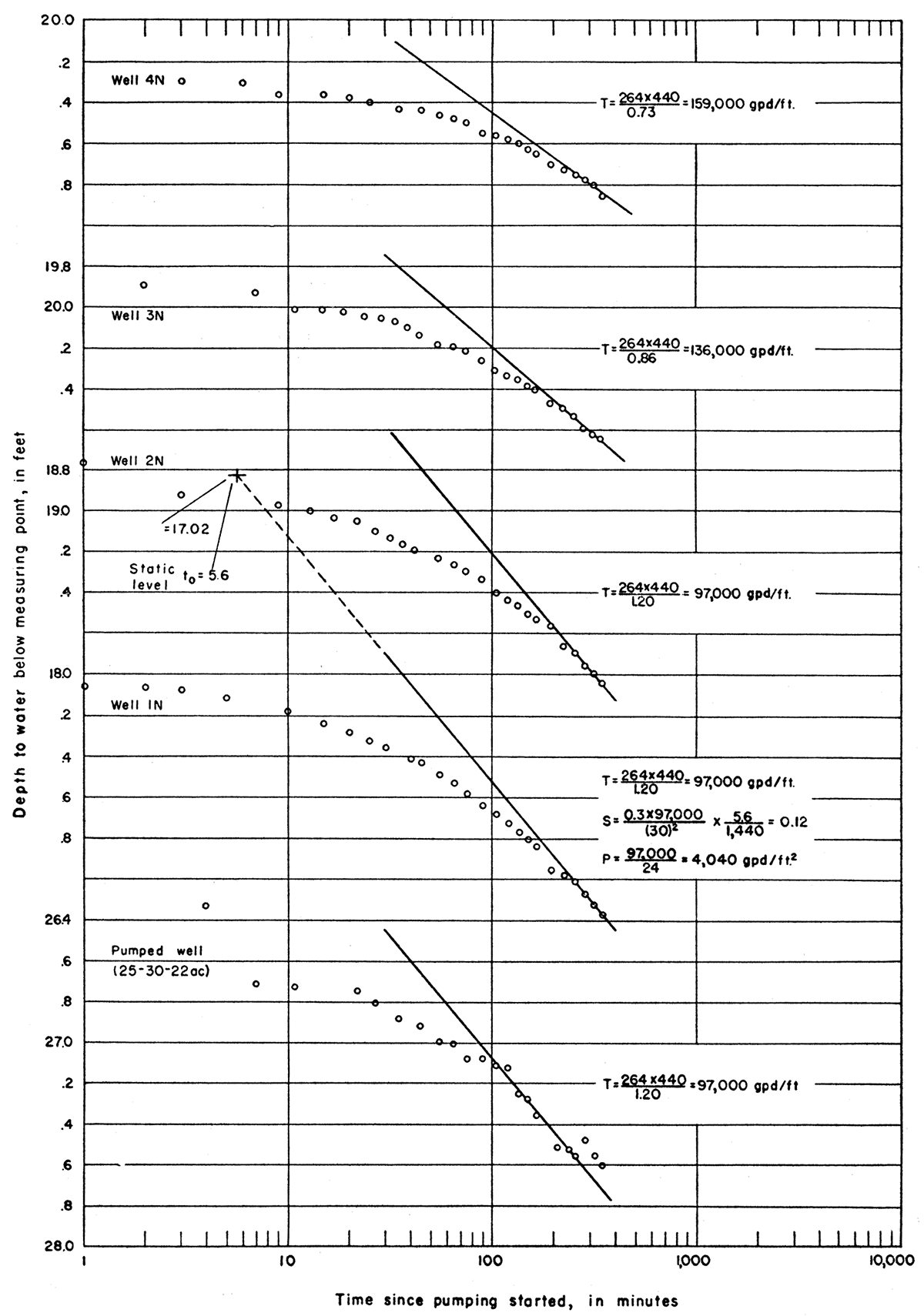
Figure 7—Drawdown of water levels in observation wells at 90 and 345 minutes during the Ven John aquifer test plotted against distance from pumped well.

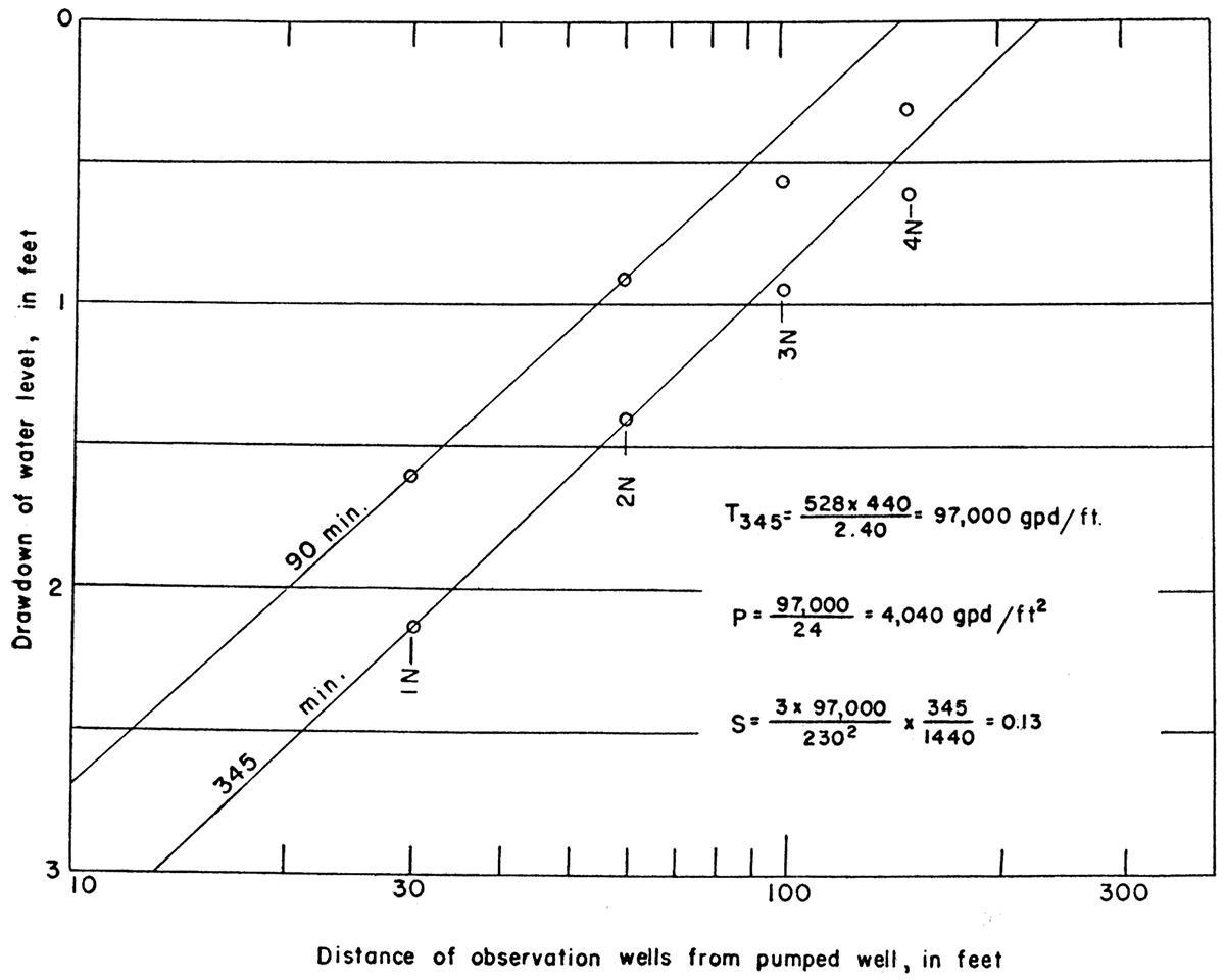
Table 2—Depth to water measured in pumped well and observation wells during Ven John aquifer test February 29, 1956.

Time since pumping started, in minutes	Depth to water below measuring point, in feet					Remarks
	Pumped well	Well 1N	Well 2N	Well 3N	Well 4N
8:10 a.m.	17.30	17.02	18.42	19.70	20.24	Static
9:05		17.03
9:15						Pump on
1		18.06	18.77
2		18.06		19.90
3		18.07	18.86		20.29
4	26.33
5		18.11
6					20.31
7	26.70			19.94
9			18.97		20.37
10		18.18
11				20.02
12	26.72
13			18.99
15		18.24		20.02	20.37
17	26.72		19.03
19				20.03
20		18.28			20.38
22	26.74		19.05
24				20.05
25		18.32			20.40
27	26.80		19.10
29				20.06
30		18.35
32			19.13
34				20.08
35	26.88				20.43
37			19.16
39				20.11
40		18.41
42			19.19
45	26.91	18.43		20.14	20.44
55	26.99	18.49	19.23	20.10	20.46
65	27.00	18.53	19.26	20.20	20.48
75	27.07	18.58	19.29	20.22	20.50
90	27.07	18.64	19.33	20.27	20.55
100	27.11	18.68	19.40	20.32	20.56
120	27.12	18.73	19.43	20.34	20.58
135	27.25	18.77	19.46	20.36	20.60
150	27.27	18.80	19.50	20.39	20.63
165	27.35	18.84	19.53	20.41	20.65
195			19.60	20.48	20.70
210	27.51
225		18.98	19.66	20.50	20.73
240	27.52
255	27.55	19.01	19.69	20.54	20.75
285	27.47	19.07	19.75	20.60	20.80
315	27.55	19.12	19.79	20.63	20.81
345	27.60	19.17	19.84	20.65	20.86

The coefficients of transmissibility shown in Figure 6 were determined by the Jacob modified nonequilibrium method. The coefficients computed from data from the pumped well and observation wells 1N and 2N are thought to be correct. Larger coefficients of transmissibility were obtained from data from observation wells 3N and 4N because pumping time was insufficient for the drawdown data to attain the correct slope. Figure 7 shows the calculation for T by the Thiem method. The coefficient of transmissibility obtained by both methods was 97,000 gpd/ft, and the coefficient of permeability was about 4,040 gpd/ft².

A storage coefficient of 0.12 was obtained by the Jacob modified non equilibrium method, and of 0.13 by the Thiem method (Fig. 6 and 7). Had the test been longer, the storage coefficient probably would have been larger than 0.13. Some drawdown occurred in all the observation wells immediately after pumping started. During the early period of the test, the aquifer acted temporarily as an artesian aquifer. The vertical permeability probably is considerably less than the horizontal permeability; the difference results in temporary artesian conditions.

The field data were not adjusted for the thinning of the aquifer during the test because it was not enough to warrant adjustment.

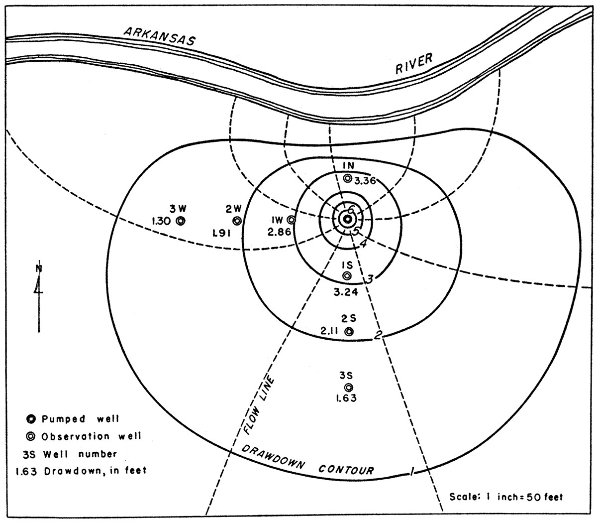
Renick—An aquifer test was made to determine the permeability of the alluvial material through which Arkansas River flows and to determine whether the water could be induced to move from the river to a pumped well adjacent to it. A well to be pumped and 7 observation wells were constructed for an aquifer test in the NE SE sec. 25, T. 25 S., R. 30 W., on the farm of Frank Renick. The respective locations of the pumped and observation wells are shown in Figure 8. The pumped well, 16 inches in diameter, 42 feet deep, and screened with perforated pipe, was drilled to the base of the alluvium 70 feet from Arkansas River. The thickness of the saturated material prior to the test was 36 feet. Holes were augered to a depth of 44 feet at the site of observation wells 1S, 3S, and SW to determine the character and depth of the alluvium. No layers of silt or clay are present in the water-bearing zone.

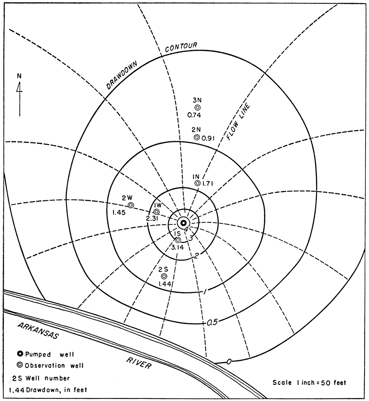
Figure 8—Contour map showing drawdown at end of aquifer test at Renick site (25-30-25da1).

The well was pumped March 14 and 15, 1956, at an average rate of 1,300 gpm. Water-level measurements made in the seven observation wells are given in Table 3. Depth to water level in the observation wells is plotted against time in Figure 9, and the drawdown of water level in the observation wells west and south of the pumped well after 60, 180, and 1,020 minutes of pumping is plotted against distance from the pumped well in Figure 10. A cross section of the test site before and after pumping is shown in Figure 11.

Table 3—Depth to water measured in observation wells during Renick aquifer test March 14-15, 1956

Time since pumping started, in minutes	Depth to water below measuring point, in feet							Remarks
	Well 1S	Well 2S	Well 3S	Well 1W	Well 2W	Well 3W	Well 1N
9:45a.m.	6.20	6.10	7.98	7.21	7.92	9.37	9.72	Static
10:25								Pump on
1		6.65	8.18			9.69	11.68
2						9.77
2.5	7.50
3			8.27		8.35	9.78	11.68
4							11.59	Reduced speed of pump motor slightly
4.5	7.64
5		6.70		8.61		9.77	11.54
6	7.81				8.65
7						9.87
8	7.89			8.86			11.84
9			8.33			9.87	11.84
10	7.94	6.84			8.72
11						9.87	11.93
12		6.87		8.88			11.93
13	7.98
14			8.39		8.74		11.97
15				9.02		9.89
16	8.04						11.99
17		6.90
20	8.10	6.94	8.44	9.05	8.81	9.89	12.04
25	8.15	7.00	8.49	9.10	8.87	9.93	12.09
30	8.20	7.03	8.50	9.13	8.89	9.94	12.12
35	8.24	7.05	8.52	9.16	8.90	9.99	12.15
40	8.29	7.10	8.56	9.18	8.93	10.01	12.17
45	8.32	7.13	8.57	9.21	8.97	10.04	12.22
50	8.35	7.15	8.59			10.05	12.23
55	8.38	7.18	8.62	9.27	9.02	10.06	12.25
60	8.41	7.20	8.64	9.30	9.05	10.08	12.27
65				9.32	9.07
70	8.47	7.25	8.68	9.35	9.08	10.07	12.32
75					9.11
80	8.51	7.30	8.73	9.39		10.12	12.35
85					9.15
90	8.57	7.35	8.77	9.43		10.15	12.40
95					9.19
100	8.61	7.38	8.78	9.45		10.16	12.42
110	8.65			9.49		10.15	12.44
125	8.69	7.44	8.86	9.54	9.26	10.17	12.50
140	8.74	7.48	8.89	9.58	9.29	10.21	12.53
160	8.80	7.53	8.94	9.63	9.33	10.22	12.56
180	8.84	7.62	8.97	9.67	9.35	10.24	12.59
210	8.90	7.68	9.05	9.72	9.39	10.28	12.61
240	8.95	7.71	9.09	9.75	9.45	10.31	12.66
270	9.00	7.77	9.13	9.80	9.48	10.34	12.69
300	9.03	7.80	9.18		9.51	10.38	12.73
330	9.06	7.84	9.22	9.85	9.53	10.39	12.76
360	9.10	7.87	9.24	9.87	9.55	10.40	12.77
420	9.15	7.92	9.33	9.92	9.60	10.44	12.83
480	9.22	7.98	9.36	9.94	9.64	10.49	12.87
540	9.24	8.00	9.39	10.00	9.69	10.53	12.90
600	9.28	8.04	9.42	10.03	9.70	10.54	12.93
660	9.31	8.07	9.46	10.05	9.72	10.57	12.95
720	9.34	8.10	9.50	10.08	9.75	10.59	12.98
780	9.36	8.13	9.51	10.11	9.77	10.60	13.01
900	9.40	8.17	9.57	10.15	9.81	10.64	13.05
1,020	9.44	8.21	9.61	10.18	9.84	10.67	13.08

Figure 9—Depth to water measured in observation wells during Renick aquifer test plotted against time since pumping started (25-30-25da1).

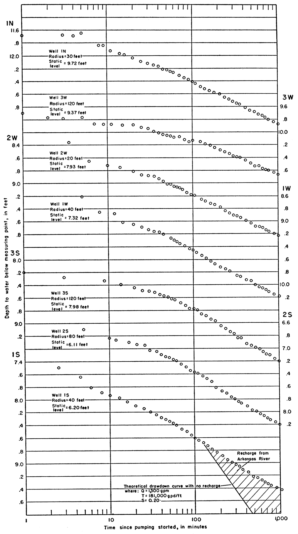
Figure 10—Drawdown of water levels in observation wells at 60, 180, and 1,020 minutes during Renick aquifer test plotted against distance from pumped well (25-30-25da1).

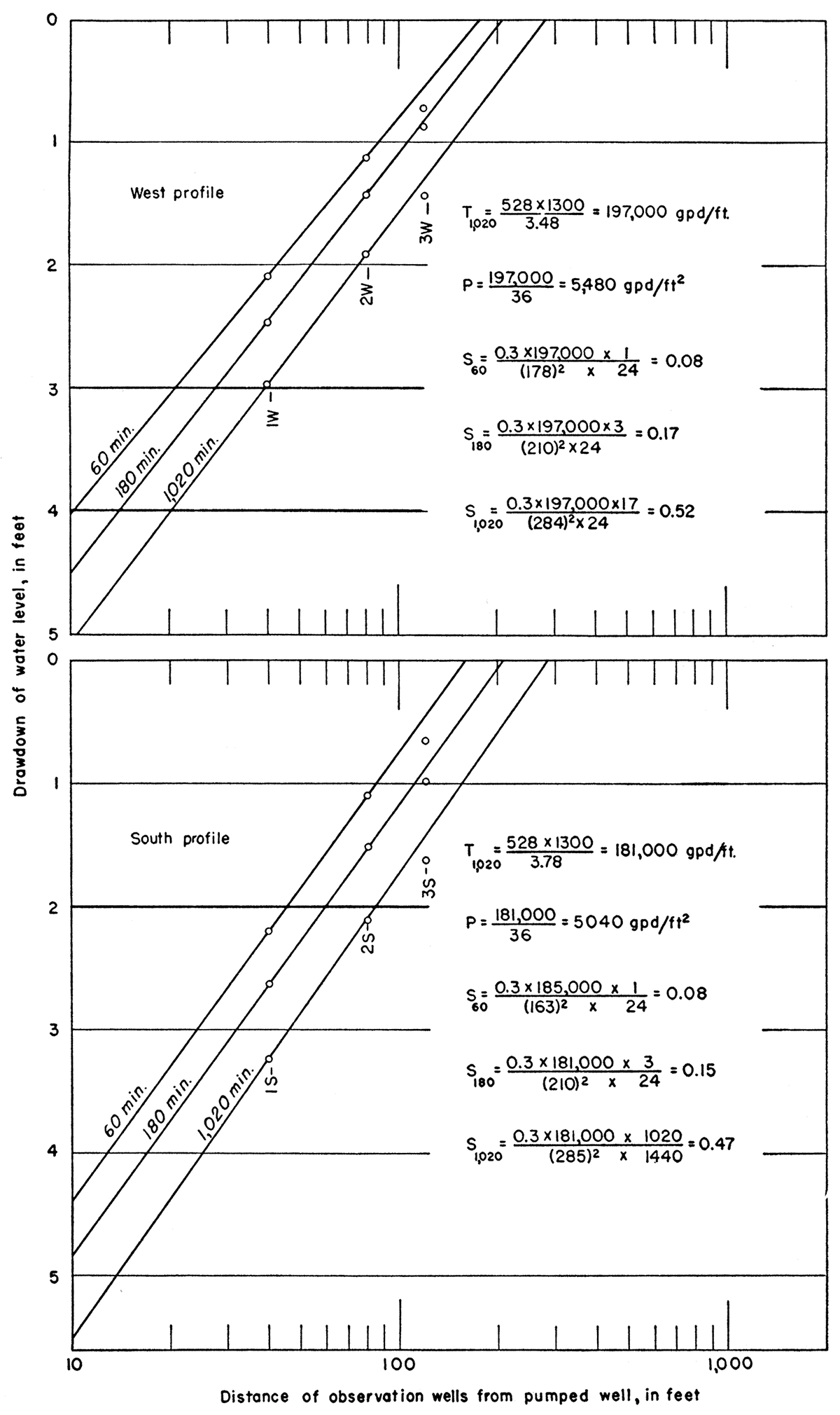
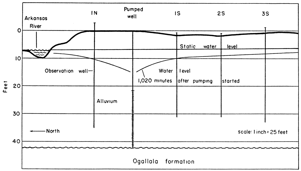
Figure 11—Cross section at Renick test site before and after pumping.

The shape of the time-drawdown curves (Fig. 9) indicates that recharge occurred during the test. If no recharge had occurred, the curves would have continued to decline until they approximated the theoretical curve shown for observation well 1S in Figure 9. In effect, the time-drawdown curves are the resultant of a curve representing drawdown caused by pumping an aquifer that has no recharge and a curve representing recovery caused by leakage from Arkansas River. The curves indicate that recharge did not occur during the early stage of the aquifer test. The downward trend of the curves representing the later stage of the test indicates that recharge was being received from Arkansas River. At the completion of the test, however, the cone of influence still was developing on the landward side, and infiltration from the river was not yet sufficient to supply the yield of the well. The curves show time lags according to the time required for recharge from the river to reach the observation wells; the time, in turn, depends on the distance of the observation wells from the river. Had the test been longer and had recharge continued to develop, the flow from the river would have continued to increase, and the proportion from storage would have continued to decrease. Eventually, nearly all the water being pumped would come from the river.

Computations of coefficients of transmissibility, permeability, and storage can be made from the time-drawdown curves only if the curves attain a constant slope prior to the beginning of recharge. In this test the recharge began before the curves had time to reach a constant slope; hence the coefficients of transmissibility and storage could not be determined from these plots.

The coefficients of transmissibility, permeability, and storage shown in Figure 10 were determined by the Thiem method. The recharge that occurred during the test did not invalidate the computations of the coefficients of transmissibility and permeability, because their values depend on the slope of the line drawn through the drawdown points, and as the effect of recharge is negligible in the early part of the tests in all observation wells, the slope of the line is not changed materially. Based on data from observation wells 1S, 2S, and 3S, perpendicular to the river, after 1,020 minutes of pumping, the coefficients of transmissibility and permeability were 181,000 gpd/ft and 5,000 gpd/ft², respectively. Approximately the same coefficients of transmissibility and permeability were obtained from drawdown data after 60 and 180 minutes. A slightly higher coefficient of transmissibility was obtained by using data from observation wells 1W, 2W, and 3W parallel to the river than by using wells 1S, 2S, and 3S perpendicular to the river; this difference probably was caused by changes in lithology within the aquifer and partially penetrating observation wells. The lower coefficient of transmissibility obtained from these data has been used.

The storage coefficients were computed after 60, 180, and 1,020 minutes of pumping. The coefficients of 0.15 and 0.17 obtained from the 180-minute data probably were not affected much by recharge, and the error caused by recharge was small. As recharge progressed, the rate of draw down decreased; hence the zero radius intercept was much less than it would have been if no recharge had occurred. S as computed from data from wells 1W, 2W, and 3W at the end of 1,020 minutes was 0.52. This high coefficient of storage also indicates recharge from the river. The storage coefficient of 0.17 percent is not necessarily correct, but probably is of the correct order of magnitude.

Leslie E. Mack has applied an analog field plotter to the groundwater How during the Renick and Norbert Irsik tests. The analog plotter consists of a power source, a voltage divider having a nullpoint indicator and probe, and a special resistance paper. Many natural phenomena such as electrostatics, magnetostatics, heat How, electric-current How, and fluid How are related in their field theory by the Laplace equation, and it can be shown that a problem in the steady-state motion of ground water is mathematically analogous to a problem in the steady-state How of electricity. This analogy between the How of electric current and the How of ground water can be demonstrated with the analog field plotter by relating electrical potential to hydraulic head. A ground-water situation can be reproduced to scale by applying How boundaries determined in an aquifer test with conductive paint on the resistance paper. Wire leads from the power supply are connected to the painted boundaries, causing a current to How through the paper. Equipotential points then are marked by the probe and connected to form the desired contour lines.

The analog plotter was used to prepare the contour map (Fig. 8) from data collected during the Renick aquifer test. The drawdown contour lines are distorted near Arkansas River because of recharge from the river. Flow lines cross the contour lines at right angles and are shown as dashed lines. These How lines mark the paths that particles of water would follow to the pumped well. Water that had its source in Arkansas River was moving toward the pumped well at the completion of the aquifer test. Figure 8 illustrates that water can be made to move from Arkansas River into the alluvium if the water table adjacent to the river is lowered below the river level.

Norbert Irsik—A second aquifer test was made to determine the permeability of the alluvial material and to determine whether the water in Arkansas River would move to a pumped well. A well for the pumping test and seven observation wells were constructed in the NE SW sec. 28, T. 25 S., R 29 W., on the farm owned by Norbert Irsik (Fig. 12). The pumped well, 16 inches in diameter, 29 feet deep, and screened with perforated pipe, was drilled to the base of the alluvium, 135 feet from Arkansas River. The thickness of the saturated material prior to the test was 22 feet; holes were augered to a depth of 35 feet at the site of observation wells 1N and 2W to determine the character and thickness of the alluvium. No layers of silt or clay are in the water-bearing zone.

Figure 12—Contour map showing drawdown at end of aquifer test at Norbert Irsik site (25-29-28ca).

The well was pumped March 21 and 22, 1956, at an average rate of 700 gpm. Water-level measurements made in the seven observation wells are given in Table 4 and are plotted against time in Figure 13; the drawdown of water level in the observation wells west and north of the pumped well after 60 and 900 minutes of pumping is plotted against distance from the pumped well in Figure 14. A cross section of the test site before and after pumping is shown in Figure 15.

Table 4—Depth to water measured in observation wells during Norbert Irsik aquifer test on March 21-22, 1956.

Time since pumping started, in minutes	Depth to water below measuring point, in feet							Remarks
	Well 1N	Well 2N	Well 3N	Well 1W	Well 2W	Well 1S	Well 2S
7:45a.m.	9.34	17.77	16.36	9.77	10.58	5.86	4.16	Static level
12:30 p.m.								Pump started
1	10.22
2						8.21
3		17.98
5			16.57	11.24
6	10.27
7		18.02			11.21
9			16.59			8.27
10	10.32
11		18.05					4.78
12			16.60	11.31
14					11.28
15	10.35
16		18.08
17			16.62			8.34
18							4.84
20	10.38
21.		18.09		11.36
22			16.63
25	10.40				11.32
26		18.91
27			16.65			8.40
28							4.92
30	10.42
31		18.12		11.41
32			16.67		11.36
40	10.47					8.46
41		18.15					4.98
42			16.70	11.47
43					11.41
50	10.50					8.52
51		18.18					5.02
52			16.70	11.51
53					11.46
60	10.54	18.20	16.72			8.56	5.07
63				11.55	11.51
75	10.57	18.22	16.73			8.59	5.11
77				11.59	11.54
90	10.61	18.25	16.75	11.63	11.56	8.63	5.16
110	10.64	18.28	16.77	11.67	11.60	8.68	5.18
130	10.69	18.32	16.81	11.72	11.65	8.71	5.28
150	10.73	18.34	16.82	11.74		8.74	5.30
180	10.77	18.39	16.87	11.80	11.69	8.79	5.36
210	10.81	18.42	16.88	11.85	11.7.5	8.82	5.40
240	10.84	18.45	16.90	11.87	11.78	8.87	5.44
300	10.89	18.49	16.95	11.91	11.80	8.90	5.46
390	10.94	18.54	17.00	11.99	11.87	8.93	5.53
480	10.99	18.58	17.03	12.01	11.94	8.96	5.55
600	11.02	18.62	17.07	12.04	11.95	8.98	5.58
720	11.04	18.64	17.08	12.06	11.98	9.00	5.59
900	11.05	18.68	17.10	12.08	12.03	9.00	5.60

Figure 13—Depth to water measured in observation wells during Norbert Irsik aquifer test plotted against time since pumping started (25-29-28ca).

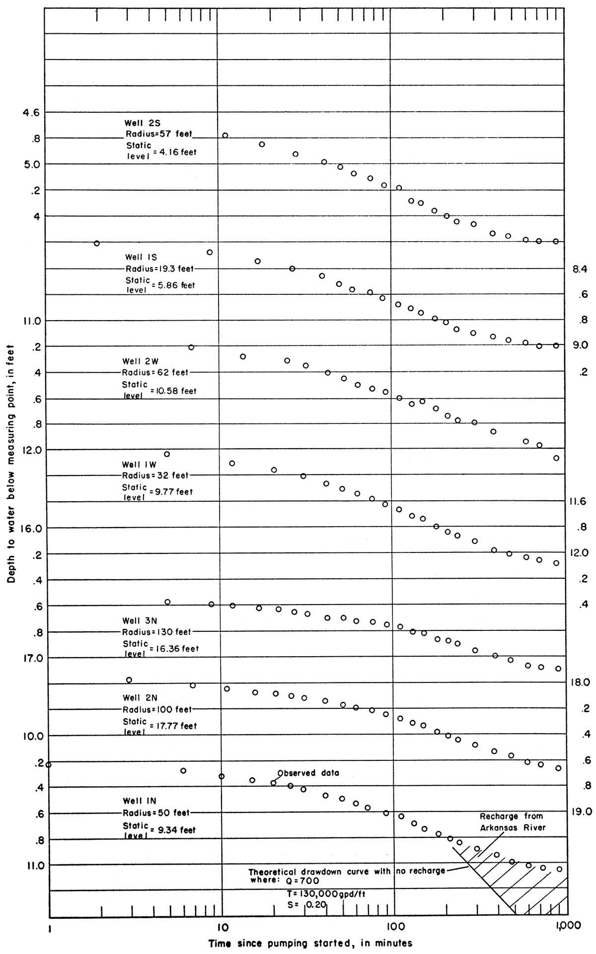
Figure 14—Drawdown of water levels in observation wells at 60 and 900 minutes during Norbert Irsik aquifer test plotted against distance from pumped well (25-29-28ca).

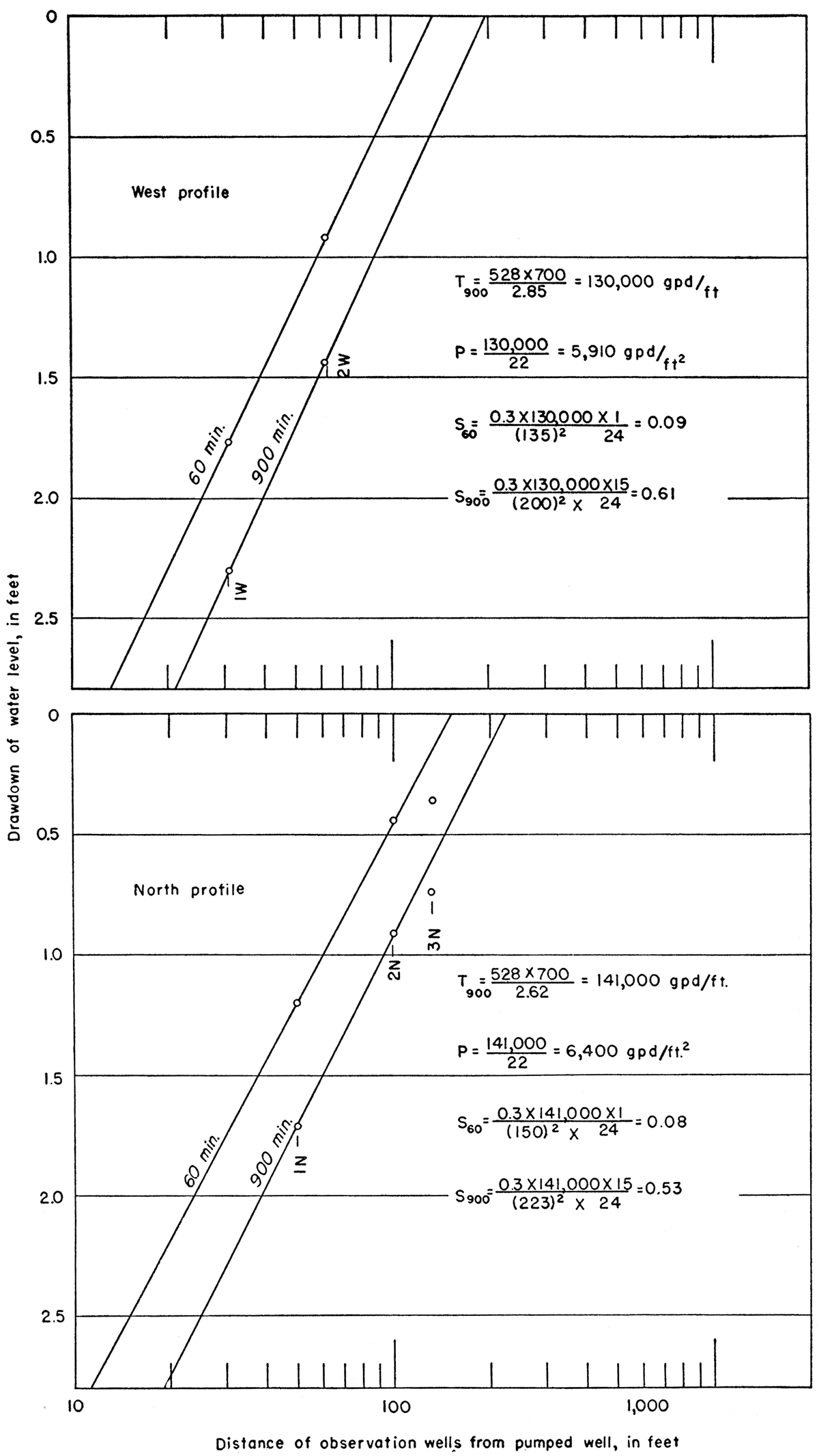
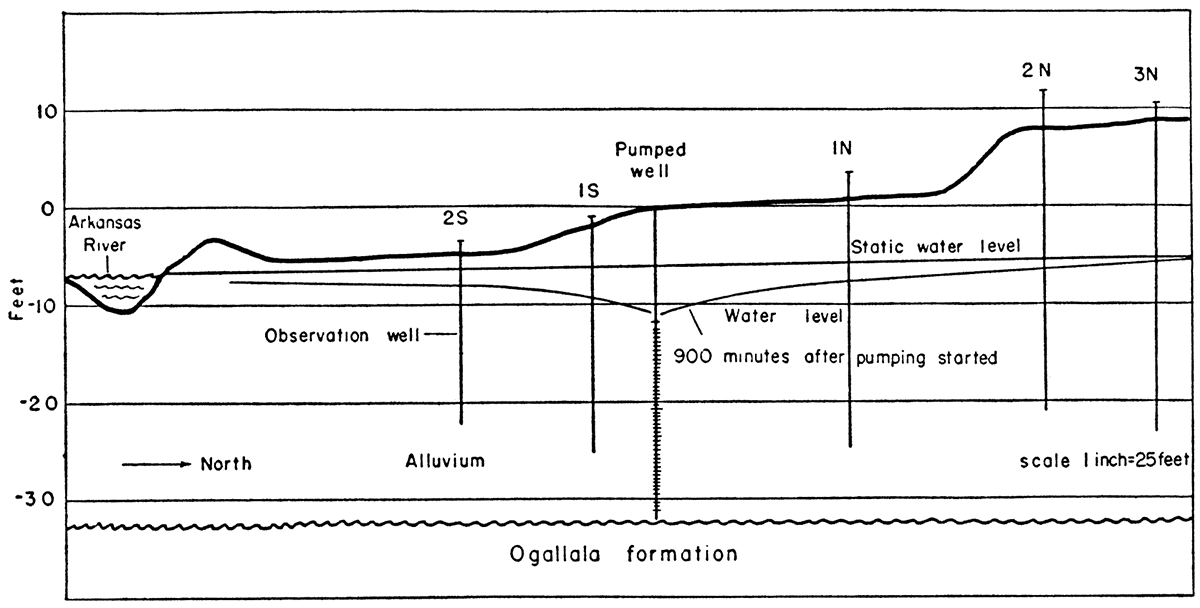
Figure 15—Cross section at Norbert Irsik test site before and after pumping.

The shape of the time-drawdown curves (Fig. 13) indicates that recharge occurred during the test. In general, this test had the same characteristics as the Renick test. The coefficient of transmissibility computed from data from observation wells 1N, 2N, and 3N at 900 minutes was 140,000 gpd/ft. (Fig. 14), which was lower than at the Renick site.

Recharge occurred before the drawdown data would plot at a constant slope, and the coefficients of transmissibility, permeability, and storage could not be determined from the plot in Figure 13. They were determined by the Thiem method and are shown in Figure 14. The smallest transmissibility coefficient was obtained from data from observation wells 1W and 2W at 900 minutes and was 130,000 gpd/ft, The coefficient of permeability was 5,900 gpd/ft².

At the end of the test, the water table along a line parallel to Arkansas River had a steeper slope than the water table along a line perpendicular to the river on the side of the well opposite from the river, as would be expected if river recharge occurred during the test. Had there been no recharge, the slope of the water table toward the river and parallel to the river would have been about the same.

The storage coefficients were computed from the observation-well data after 60 and 900 minutes of pumping. The coefficients obtained after 60 minutes were 0.08 and 0.09 as compared to 0.53 and 0.61 after 900 minutes. The high storage coefficients of 0.53 and 0.61 also indicate that recharge from the river occurred. None of the storage coefficients was judged to be valid.

The analog plotter was used to prepare the contour map (Fig. 12) from data collected during the Norbert Irsik aquifer test. The fact that drawdown contour lines are distorted near Arkansas River because of recharge from the river demonstrates that water can be made to move from Arkansas River into the alluvium if the water table adjacent to the river is lowered below the river level.

Tests in Ogallala Formation Underlying Alluvium

McGehee—A well to be pumped and seven observation wells were constructed in the SE NW sec. 21, T. 25 S., R. 30 W., on the farm of Myles McGehee to test the Ogallala formation underlying the alluvium. The pumped well was drilled through the Ogallala formation to a depth of 162 feet and was cased with 16-inch casing that was machine slotted at a depth of 82 to 162 feet. A 45-foot length of 26-inch surface casing was set around the 16-inch casing to seal out the water in the alluvium.

Observation wells 1N, 2N, 3N, and 4N were drilled in a line extending north from the pumped well at distances of 100, 200, 300, and 400 feet, respectively. The observation wells were completed with 2-inch casing at the same depth and were screened in the same zones as the pumped well. A 45-foot length of 6-inch surface casing was set around the 2-inch casing to seal out the water in the alluvium. The observation wells were developed by compressed air.

Three observation wells were completed in the alluvium at distances of 38, 70, and 100 feet east of the pumped well. These wells were used to note any decline of water level in the alluvium, but no decline was noted throughout the test; hence the field data have not been included in the report.

The well was pumped at an average rate of 360 gpm for 26 hours by means of a turbine pump powered by a butane motor. The yield of the well was held constant by regulating the speed of the motor. Water-level measurements were made in the seven observation wells and the pumped well. The data obtained in the pumped well and the four observation wells finished in the Ogallala formation are given in Table 5. Water samples were taken from the pumped well at intervals during the test.

Table 5—Drawdown and recovery of water levels in pumped well and observation wells during McGehee aquifer test July 23-24, 1956.

Time since pumping started, in minutes	Drawdown, in feet
	Pumped well	Well 1N	Well 2N	Well 3N	Well 4N
1.5		1.29	0.13
2.5		2.33	0.53
3.5		3.24	1.03
4.5		4.08	1.45
5.5		4.86	1.83
6		5.25
7		6.02	2.35	1. 35	0.27
8		6.70	2.87		.36
9		7.33	3.23		.59
10		7.86	3.59	1.73	.70
11		8.36	3.92	2.42	.86
12		8.80	4.25	2.69
13		9.28	4.52		1.07
14		9.53	4.78
15		9.84	5.03		1.33
16		10.12	5.25	3.47
17		10.38	5.46	3.67	1.57
18		10.60	5.66	3.85
19		10.80	5.83
20		11.02	6.02	4.13	1. 90
21		11.17	6.27	4.27
22		11.42	6.30	4.39	2.11
23		11.60	6.88	4.54
24	42.19		7.16	4.67	2.29
25		11.91	7.31	4.77
26			7.53	4.87	2.32
27		12.22		4.98
28			7.63	5.10	2.64
29		12.47		5.20
30	42.92		7.78	5.32	2.79
31		12.70		5.41
32			7.91	5.49
33		12.89
34			8.04
35		13.07		5.75	3.04
36			8.18
37		13.28
38			8.33
39		13.70		6.07
40	43.73		8.47	6.14	3.54
42			8.62	6.25
44		13.88	8.74	6.40
45		13.96			3.86
46			8.87	6.42
47				6.51
48		14.17		6.64
49			9.04
50	44.18			6.76	4.13
51		14.39
52			9.21
54		14.58		6.97
55			9.37		4.43
57		14.73
58			9.50	7.17
60	44.74	14.93	9.63		4.63
62				7.37
64		15.15
65			9.83	7.41	4.88
68		15.41
70			10.09	7.83	5.09
72		15.60
75		15.74	10.29	7.94	5.31
78	46.00
80		15.95	10.47	8.13	5.51
85		16.14	10.66	8.30	5.67
90		16.42	10.83	8.31	5.86
95		16.53	11.03	8.61	6.02
100		16.74	11.21	8.77	6.21
105	47.26	16.89	11.38	8.94	6.36
110		17.01	11.54
112				9.09
115		17.15			6.60
117			11.75	9.25
120	47.39	17.32
123			11.89
125				9.46
127					6.94
130		17.52
133			12.13
135	47.41			9.66
137					7.17
140		17.60	12.22
145				9.79	7.33
150	47.52	17.97	12.41
160		18.15	12.64	10.12	7.64
170		18.32	12.78	10.39	7.81
180	47.73	18.43	12.90	10.52	8.00
195		18.68	13.10	10.87	8.24
210	48.55	18.93	13.29	10.97	8.45
225		19.15	13.47	11.18	8.64
240	48.81	19.25	13.59	11.40	8.83
260		19.54	13.83	11.56	9.06
280		19.67	13.95	11.74	9.25
300	49.34	19.83	14.08	11.91	9.45
330		20.00	14.25	12.13	9.70
345	49.80
360		20.29	14.46	12.33	10.01
390		20.39	14.58	12.47	10.20
405	50.09
420		20.60	14.73	12.67	10.36
450		20.78	14.88	12.86	10.58
465	50.35
480		20.83	14.96	12.95	10.75
510	50.93
540		20.96	15.12	13.17	11.03
585	51.21
600		21.30	15.38	13.39	11.23
660	51.39	21.58	15.59	13.60	11.50
720		21.67	15.68	13.77	11.66
780	51.42	21.64	15.71	13.83	11.75
900	51.80	22.21	16.10	14.27	12.15
1,020	52.10	22.28	16.16	14.36	12.37
1,140	52.49	22.44	16.33	14.56	12.55
1,260	52.84	22.64	16.48	14.73	12.73
1,380	53.32	22.97	16.83	14.92	12.76
1,500	53.47	23.19	16.90	15.10	13.12
Time since pumping stopped, in minutes	Recovery, in feet
	Pumped well	Well 1N	Well 2N	Well 3N	Well 4N
0.5		0.71	0.01	0.00
1	29.18
1.5		2.87	.33
2	32.07			.22
2.5		4.27	.98		0.04
3	34.02			.50
3.5		5.32	1.63		.16
4	35.57			.81
4.5		6.21	2.21		.22
5	36.77	6.59	2.55		.29
6	37.75	7.30	2.96	1.37	.48
7	38.55	7.87	3.40		.56
8	39.26	8.36	3.80	1.93	.69
9	39.83	8.81	4.14		.83
10	40.33	9.20	4.43	2.39	.97
11	40.79
12	41.21	9.90	5.04	2.81	1.23
13	41.57
14	41.88	10.50	5.52	3.17	1.49
15	42.16
16		11.01	5.95	3.64	1.73
17	42.53
18		11.47	6.32	3.86	1.95
19	43.05
20		11.85	6.65		2.18
21	43.56			4.28
22					2.42
23		12.38	7.09
24	44.11			4.67	2.55
26		12.82	7.48		2.64
27	44.57			5.01
28					2.98
29		13.22	7.80
30	44.98			5.33	3.06
32		13.59	8.12
35	45.54	13.91	8.40	5.80	3.46
40	45.98	14.39	8.80	6.23	3.81
45	46.40	14.81	9.16	6.60	4.12
50	46.72	15.18	9.48	6.85	4.46
55	47.04	15.52	9.77	7.28	4.76
60	47.22	15.82	10.03	7.52	5.02
70	47.93	16.36	10.50	8.05	5.60
80	48.25	16.82	10.89	8.47	5.02
90	48.61	17.21	11.23	8.86	5.39
105	49.04	17.73	11.68	9.36	5.93
120	49.41	18.15	12.04	9.79	6.42
140	49.83	18.62	12.46	10.28	7.00
160	50.16	19.03	12.80	10.70	7.50
180	50.44	19.36	13.09	11.11	7.92
200	50.79
210		19.79	13.47	11.49	8.48
240	5l.05	20.11	13.7.5	11.86	8.93
270	5l.49	20.40	13.99	12.17	9.33

The drawdown of the water levels in the observation wells is plotted against time on semilogarithmic paper (Fig. 16); the recovery of the water levels is plotted against time on logarithmic paper (Fig. 17). The recovery of water levels in the observation wells and the pumped well is plotted against time on semilogarithmic paper (Fig. 18). The drawdown of the water levels in the observation wells at the end of the pumping period is plotted against the distances from the pumped well (Fig. 19). The computations for the coefficients of transmissibility and storage are included in the illustrations.

Figure 16—Drawdown of water levels in pumped well (25-30-21bd) and observation wells during McGehee aquifer test plotted against time since pumping started.

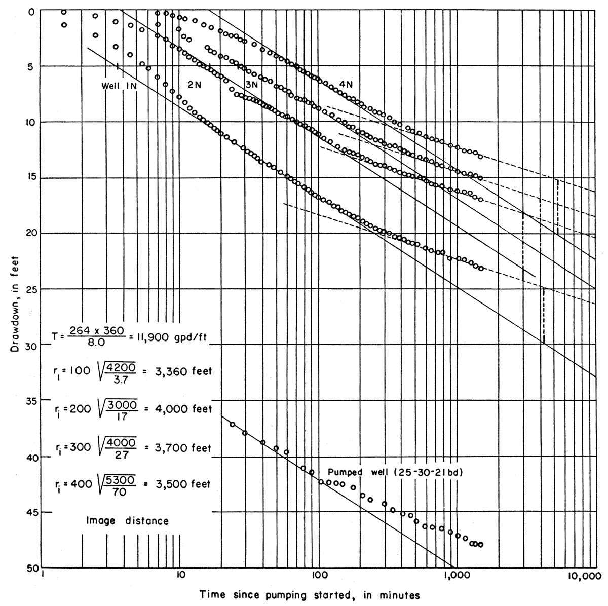
Figure 17—Recovery of water levels in observation wells during McGehee aquifer test plotted against time since pumping stopped (25-30-21bd).

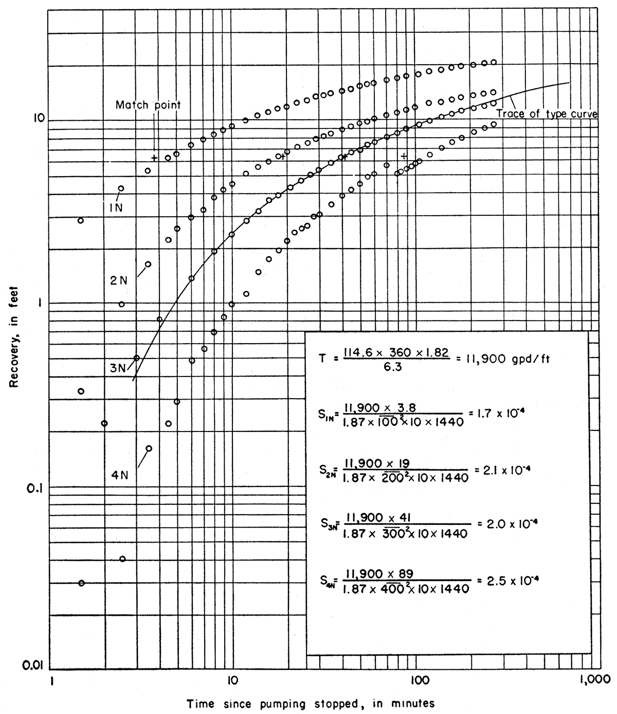
Figure 18—Recovery of water levels in pumped well and observation wells during McGehee aquifer test plotted against time since pumping stopped (25-30-21bd ).

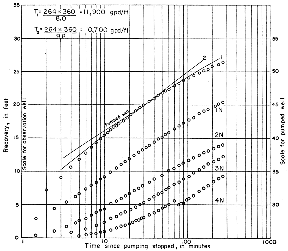
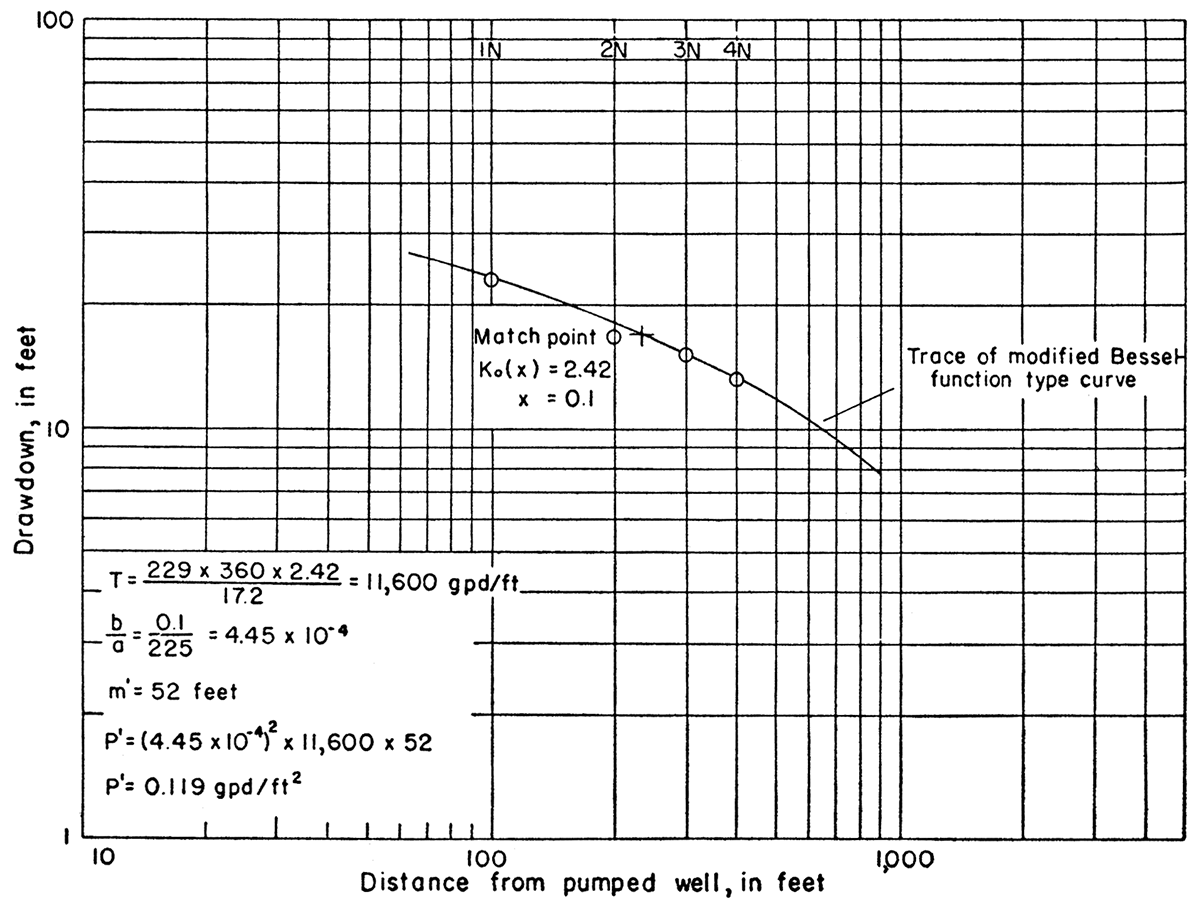
Figure 19—Drawdown of water levels in observation wells at end of McGehee aquifer test plotted against distance from pumped well (25-30-21bd).

The coefficients of transmissibility and storage shown on Figure 17 were computed by the Theis nonequilibrium method. The recovery data fit the Theis type curve very well. The match between the type curve and the observed data defines the coefficients of transmissibility and storage of the Ogallala formation at this site. The coefficient of transmissibility of the Ogallala formation was 11,900 gpd/ft., and the coefficient of storage was about 2 x 10^-4.

The recovery data of the pumped well theoretically should plot as a straight line on semilogarithmic paper by the Jacob modified nonequilibrium method, but in this test they depart in the latter part of the recovery period (Fig. 18). The recovery data from the pumped well have been computed to show two interpretations. One interpretation gives a coefficient of transmissibility of 11,900 gpd/ft, which conforms with the answer obtained by analyzing the observation-well data. The other interpretation gives a coefficient of transmissibility of 10,700 gpd/ft, which is too low. In general, the plot of the recovery data from the pumped well has the same appearance as that from the observation wells.

Figure 16 shows that the plotted drawdown data depart from the type curve in the latter part of the test. This departure may be caused by leakage from the confining bed that overlies the artesian zone in the Ogallala formation from which water was being pumped, or it may be caused by an increase in aquifer thickness and transmissibility, or by both.

The assumed leakage that caused the observed data to depart from the type curve was analyzed by the Jacob leaky-aquifer method. In Figure 19 are given the computations for the coefficient of transmissibility of the artesian aquifer and the coefficient of the vertical permeability of the confining bed. If the coefficient of the vertical permeability of the confining bed, 0.119 gpd/ft², is in error, it is probably too large. The data show that the Ogallala formation at this site has low permeability.

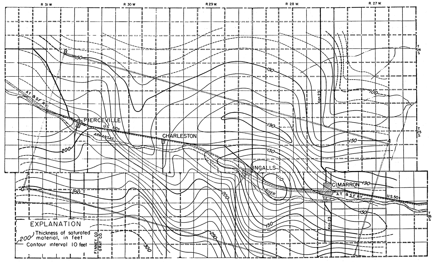
The upward deflection from the straight line shown in Figure 16 probably is caused by an increase in aquifer thickness. The increase is not abrupt, but is gradational over a large area, as shown by the saturated-thickness map (Fig. 20). The effective distance to a recharging "boundary" caused by a change to greater aquifer thickness and higher transmissibility can be determined by the following formula:

r_i = r √(t_i / t_p)

where r₁ = distance from image well to observation well, in feet,
r = distance from pumped well to observation well, in feet,
t_p = time since pumping began for a particular value of s to be observed before the boundary becomes effective, in minutes, and
t_i = time since pumping began when the divergence of the drawdown curve from the straight line under the influence of the image well is equal to the value of s at t_p, in minutes.

The close clustering of the image distances given in Figure 16 implies that the recharging boundary is caused by an increase in aquifer thickness and transmissibility. The bedrock contour map (Fig. 5) and the saturated thickness map (Fig. 20) indicate that the recharging boundary is south of the pumped well.

Figure 20—Saturated thickness of Pliocene and Pleistocene deposits in Ingalls area.

No change in chemical quality of the water pumped from the Ogallala formation was noted during the test; hence these data have not been included in the report.

Norbert Irsik—A well to be pumped and seven observation wells were constructed in the SE NW sec. 28, T. 25 S., R. 29 W., on the farm of Norbert Irsik, to test the Ogallala formation underlying the alluvium. This aquifer test was very similar to the McGehee test. The well was cased with 16-inch casing that was machine slotted at a depth of 90 to 187 feet. A 65-foot length of 26-inch surface casing was set around the 16-inch casing to seal out the water in the alluvium.

Observation wells 1W, 2W, 3W, and 4W were drilled in a line extending west from the pumped well at distances of 100, 200, 300, and 400 feet, respectively. They were completed with 2-inch casing at the same depth and were screened in the same zones as the pumped well. A 65-foot length of 6-inch surface casing was set around the 2-inch casing to seal out the water in the alluvium. The observation wells were developed by compressed air.

Three observation wells were completed in the alluvium at distances of 38, 70, and 100 feet north of the pumped well. These wells were used for measuring any decline of water level in the alluvium. As in the McGehee test, the water levels in these wells did not decline during the test; hence the data have not been included in this report.

The well was pumped at a rate of 720 gpm for 24.5 hours with the turbine pump and butane motor used in the McGehee test. Water levels were measured in the seven observation wells and the pumped well. The data obtained in the pumped well and the four observation wells finished in the Ogallala formation are given in Table 6. Water samples were taken from the pumped well at intervals during the test.

Table 6—Drawdown and recovery of water levels in pumped well and observation wells during Norbert Irsik aquifer test August 8-9, 1956

Time since pumping started, in minutes	Drawdown, in feet
	Pumped well	Well 1W	Well 2W	Well 3W	Well 4W
1.0		1.01	0.08
1. 5					0.01
2.0		2.39	.35
2.1				0.17
2.5					.02
3.0		3.63	.77
3.1				.44
3.5					.05
4.0		4.88	1.29
4.1				.88
4.5					.14
5.0		5.88	1.84
5.1				1.36
5.5					.24
6.0		6.76	2.36	1.90
7.0		7.44	2.85	2.46	.35
8.0		8.07	3.30	3.01
8.5					.49
9		8.59	3.71	3.48
9.5					.83
10		8.99	4.11	4.00
11					1.10
12		9.91	4.87		1.28
13				5.15	1.45
14		10.68	5.49	6.40	1.63
16		11.28	6.06		1.99
18		12.00	6.58		2.33
19			7.12	6.79	2.50
20		12.81			2.67
22		13.39			3.01
23			7.85
24		13.70		8.10	3.35
26		14.12	8.48		3.65
27				9.45
28					3.94
29	46.34		9.00
30		14.79		9.57	4.23
32		14.89	9.49		4.63
34		15.20
35			9.92
36		15.76		10.16	5.01
39		16.24
40			10.68		5.49
41		16.52		10.90
44		16.86
45			11.28		5.94
46		17.14		11.55
49	49.10	17.47
50			11.94	12.10	6.53
51		17.68
54		18.23
55			12.50	12.72	7.00
56		18.51
59	51.54	18.88
60			12.92	13.35	7.47
62		19.22
65		19.50	13.24	13.73	7.91
69		19.86
70			13.73	14.30	8.31
74	52.41	20.22
75			14.21	14.58	8.70
79		20.61
80			14.57	15.18	9.06
85		20.99	14.87	15.51	9.38
90	53.80	21.42	15.28	15.92	9.72
100	54.38	22.04	16.02	16.53	10.31
110		22.87	16.61	17.23	10.87
115		23.21
120	55.97	23.30	17.17	17.75	11.40
135		24.01	17.83	18.46	12.10
150	56.60	24.66	18.37	19.36	12.69
165		25.16	18.80	19.71	13.20
180	57.62	25.75	19.27	20.08	13.68
200		26.30	19.77	20.81	14.30
220	58.74	26.82	20.22	21.34	14.79
240		27.09	20.76	21.77	15.18
270	59.98	28.27	21.64	22.72	15.94
300	61.05	28.84	22.11	23.15	16.54
330	61.12	29.29	22.60	23.81	17.07
360	61.70	29.75	23.01	24.15	17.53
390	61.82	30.06	23.39	24.72	17.91
420	62.35	30.46	23.63	24.89	18.27
450	63.00	30.95	24.07	25.50	18.63
495		31.25	24.53	25.98	19.14
540	63.48	31.76		26.35	19.54
600	64.75	32.31	25.36	26.99	20.06
660		32.86	25.86	27.50	20.48
720	65.14	33.36	26.30	28.00	21.17
780	65.95	33.56	26.58	28.15	21.37
840	66.72	34.14	27.00	28.70	21.64
900		34.14	27.09	28.81	22.01
960	67.02	34.58	27.46	29.18	22.22
1,080	67.16	35.14	27.95	29.66	22.73
1,200		35.53	28.32	30.02	23.22
1,320		35.44	28.35	30.02	23.34
1,350	68.33
1,380		36.05	28.64	30.32	23.52
1,440	68.45	36.10	28.77	30.45	23.71
1,500		36.24	28.84	30.55	23.79
Time since pumping stopped, in minutes	Recovery, in feet
	Pumped well	Well 1N	Well 2N	Well 3N	Well 4N
1	34.77	2.38	0.09	0.09
2	38.11	4.41	.66	.59	0.01
3	39.88	5.82	1.29	1.20	.08
4	40.91	6.95	1.88	1.83	.19
5	41.99	7.88	2.44	2.44	.35
6	42.65		2.95	3.01	.54
7	43.44		3.43	3.53	.74
8	44.08		3.92	4.05	.94
9	44.65		4.28	4.52	1.16
10	45.15	10.42	4.69	4.96	1.38
11		10.56	5.25	5.41	1.61
12	46.01	10.72	5.42	5.74	1.82
13			5.75	6.15	2.02
14	46.74	12.44	6.08	6.51	2.24
15		13.13		6.84	2.45
16	47.35	13.70	6.67	7.15	2.69
17				7.44	2.85
18	47.94		7.23	7.74	3.02
19				8.01	3.20
20	48.40	14.22	7.73	8.25	3.38
21				8.52
22	48.91	14.77	8.21	9.00	3.74
24			8.68	9.23	4.07
25	49.55	15.43
26			9.08	9.67	4.40
28	50.13	16.00	9.46	10.07	4.71
30		16.39	9.82	10.45	5.00
31	50.64
32		16.76	10.16	10.79	5.29
34	51.00		10.48	11.13	5.56
35		17.26
36			10.79	11.47	5.82
37	51.41	17.57
38			11.09	11.77	6.07
40	51.88	18.05	11.36		6.32
42		18.29		12.07
45	52.43	18.73	12.02		6.88
47		19.10		12.75
50	53.00	19.29	12.60		7.40
53		19.61		13.37
55	53.50	19.89	13.13	13.92	7.88
60	53.95	20.31	13.63	14.49	8.34
65	54.37	20.84	14.11	14.92	8.76
70	54.76	21.23	14.49	15.41	9.18
75	54.98	21.64	14.88	15.87	9.54
80	55.50		15.25	16.25	9.88
85	55.75	22.23	15.60	16.65	10.21
90	56.05	22.73	15.94	16.97	10.52
95	56.40
100	56.65	23.39	16.53	17.59	11.10
110	57.20	23.92	17.08	18.22	11.66
120	57.75	24.56	17.59	18.72	12.12
130		24.87	18.04	19.24	12.57
140	58.50	25.34	18.47	19.70	12.99
150	58.85	25.74	18.86	20.13	13.39
160	59.23	26.12	19.23	20.52	13.76
170	59.53	26.46	19.57	20.85	14.13
180	59.84	26.79	19.89	21.23	14.39
193	60.15

The drawdown of the water levels in the observation wells is plotted against time on semilogarithmic paper (Fig. 21). The recovery of the water levels in the observation wells is plotted against time on logarithmic paper (Fig. 22). The recovery of water levels in the observation wells and the pumped well is plotted against time on semilogarithmic paper (Fig. 23). The drawdown of water levels in the observation wells at the end of the pumping period is plotted against the distance from the pumped well (Fig. 24). The computations for the coefficients of transmissibility and storage are included in the illustrations.

Figure 21—Drawdown of water levels in pumped well (25-29-28bd) and observation wells during Norbert Irsik aquifer test plotted against time since pumping started.

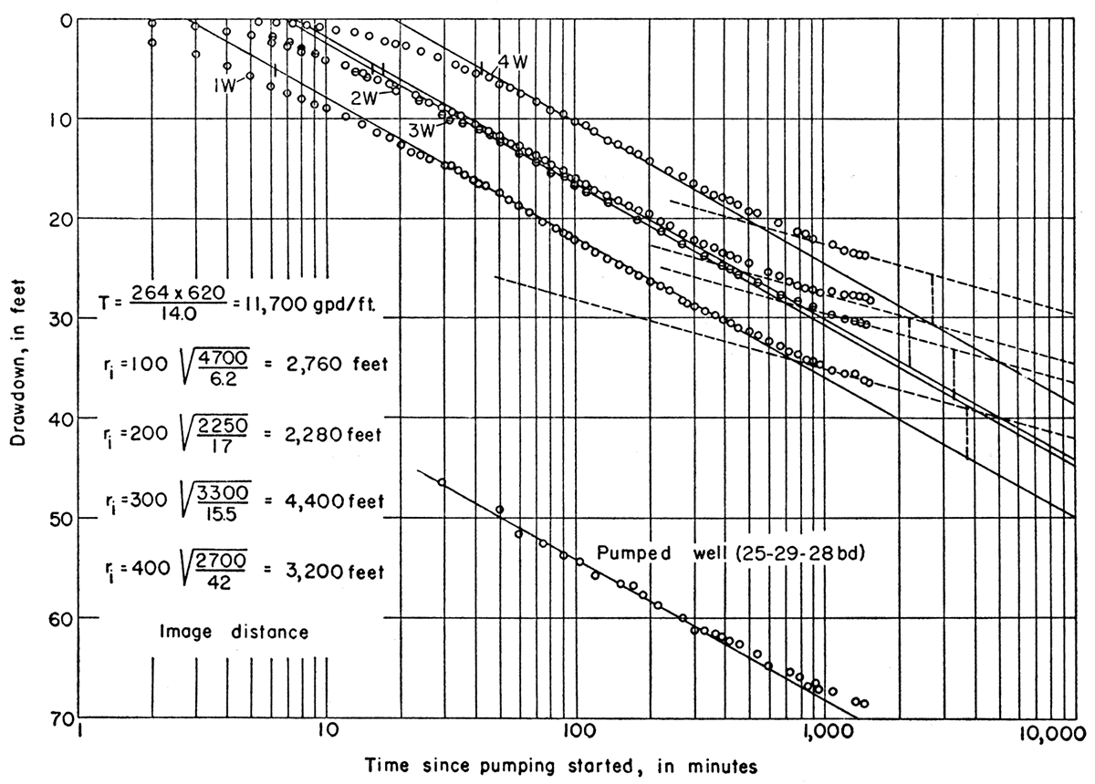
Figure 22—Recovery of water levels in observation wells during Norbert Irsik aquifer test plotted against time since pumping stopped (25-29-28bd).

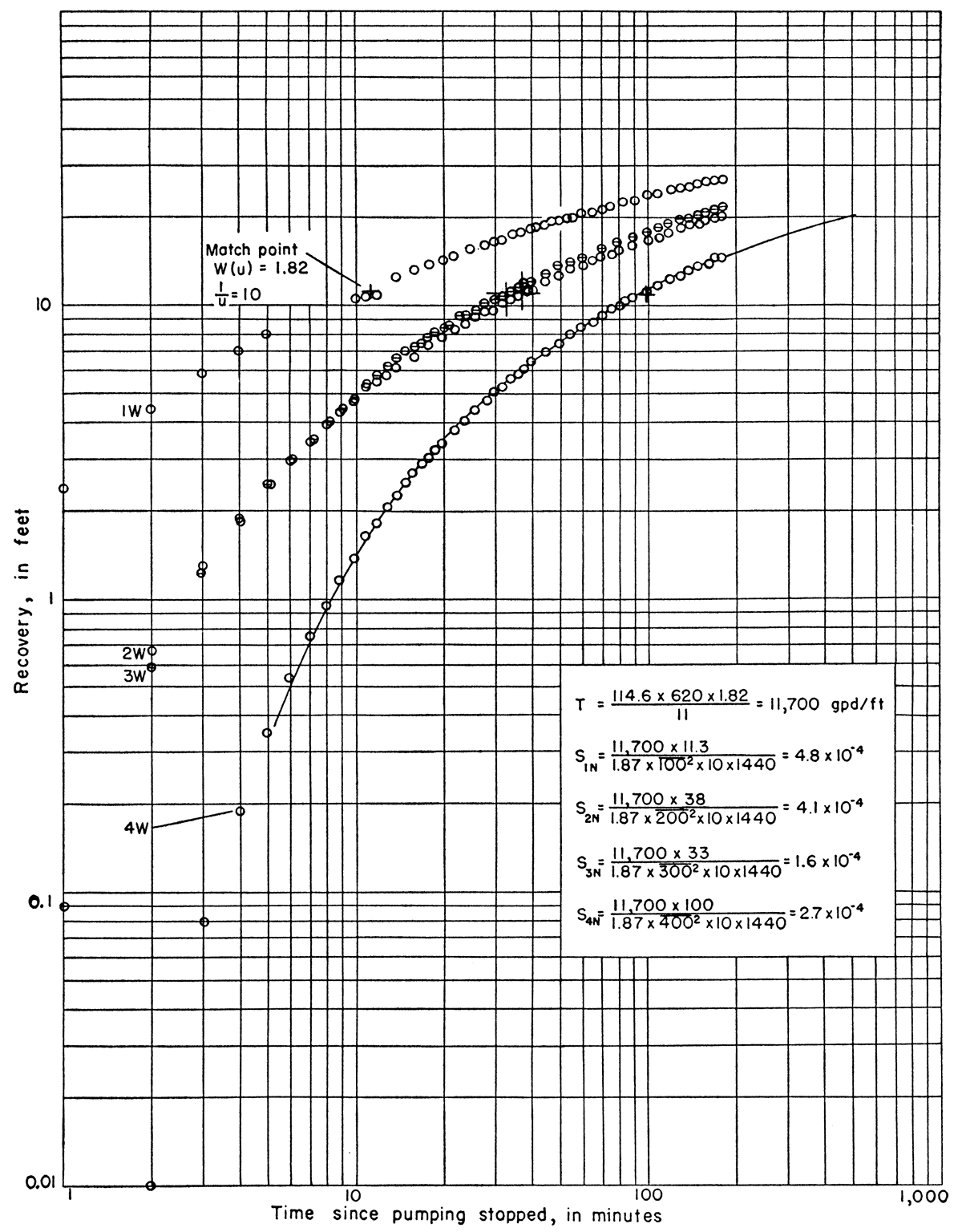
Figure 23—Recovery of water levels in pumped well (25-29-28bd) and observation wells during Norbert Irsik aquifer test plotted against time since pumping stopped.

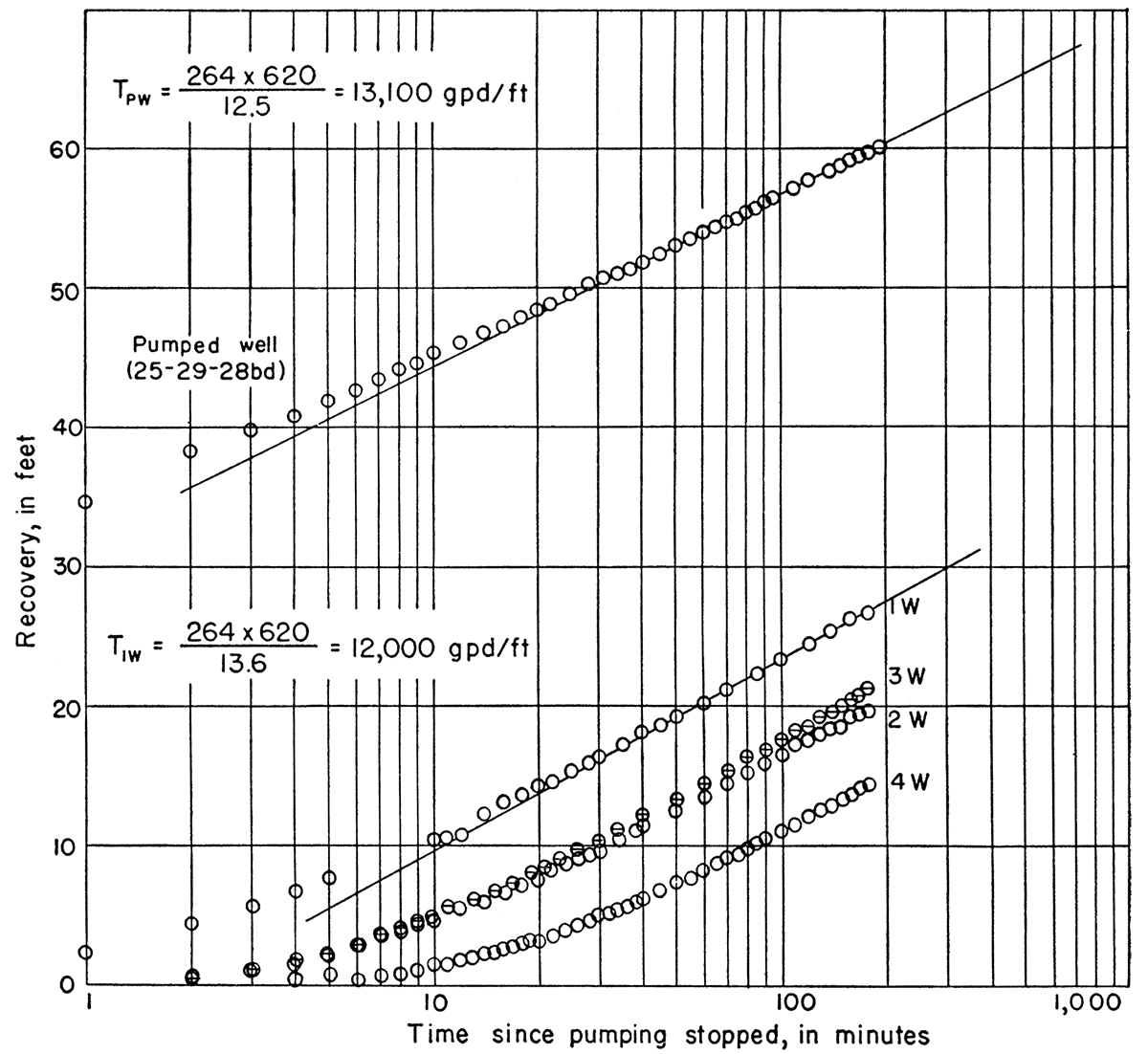
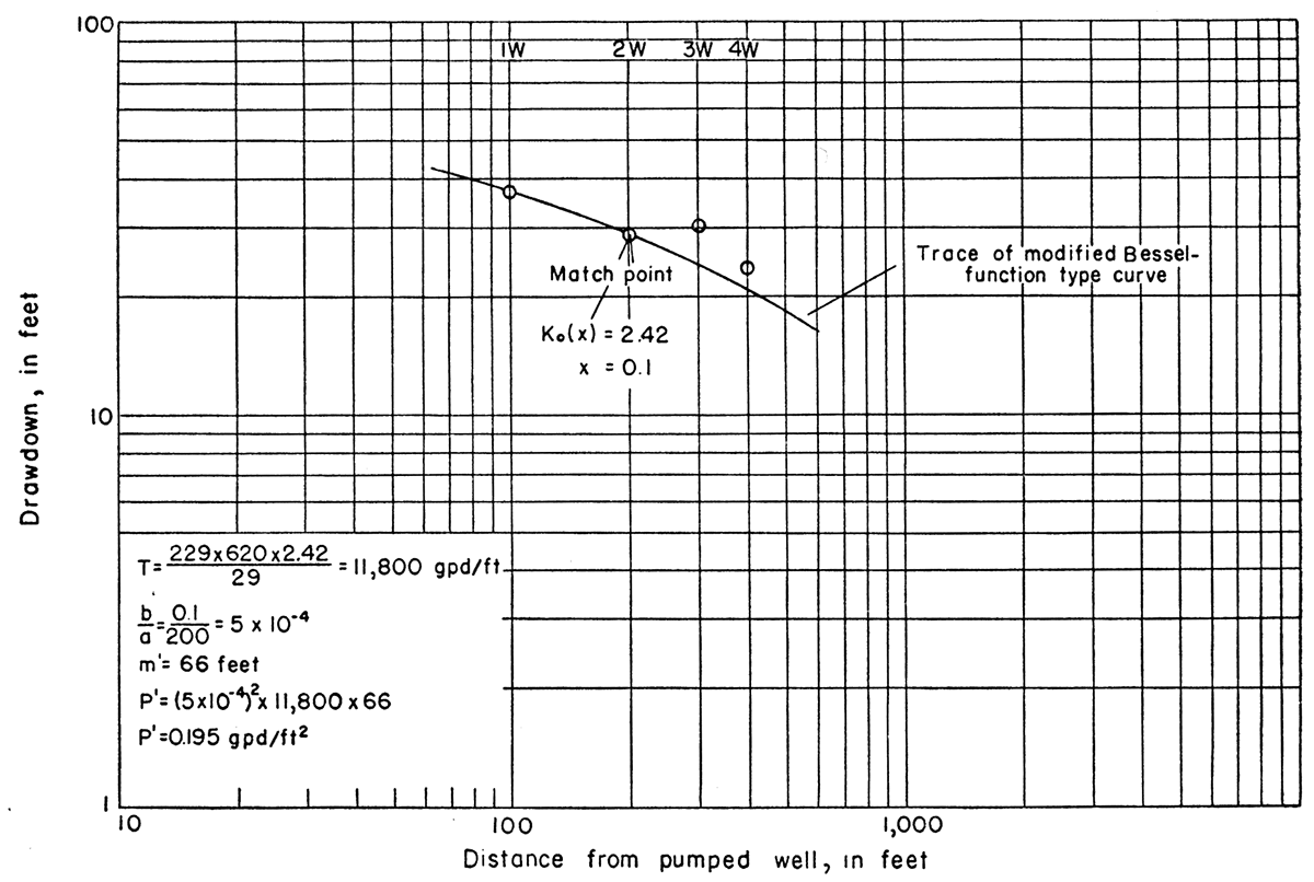
Figure 24—Drawdown of water levels in observation wells at end of Norbert Irsik aquifer test plotted against distance from pumped well (25-29-28bd).

The coefficients of transmissibility and storage shown in Figure 22 were obtained by the Theis nonequilibrium method. The recovery data fit the type curve very well. The match between the type curve and the observed data defines the coefficients of transmissibility and storage of the Ogallala formation at this site. The coefficient of transmissibility of the Ogallala formation was 11,700 gpd/ft, and the coefficient of storage was about 3 x 10^-4.

The recovery data of the pumped well plotted reasonably close to a straight line by the Jacob modified nonequilibrium method. The coefficient of transmissibility was slightly larger than that obtained from the measurements in the observation wells. The plot of the recovery data from the pumped well has the same general appearance as that from the observation wells.

Figure 21 shows that the plotted curve of the drawdown data departs from the type curve for the latter part of the test. This departure may be caused by leakage from the confining bed that overlies the Ogallala formation from which water was being pumped, or by an increase in aquifer thickness and transmissibility, or both. The leakage phenomenon was analyzed by the Jacob leaky-aquifer method. In Figure 24 are given the computations for the coefficients of transmissibility of the artesian aquifer and the coefficient of the vertical permeability of the confining bed. The coefficient of vertical permeability of the confining bed was 0.195 gpd/ft².

The upward deflection from the straight line shown in Figure 21 probably is caused by an increase in aquifer thickness to the south. The image arc distances computed for the Norbert Irsik test were not as consistent as those computed in the McGehee test, which probably were caused by a change in the lithology of the Ogallala formation.

No change in chemical quality of the water pumped from the Ogallala formation was noted during the test.

Tests in Ogallala Formation in the Upland

Clark—An aquifer test of the Ogallala formation was made by pumping an irrigation well in the NE SW sec. 32, T. 24 S., R. 30 W., on the farm leased by Lester Clark. The well, cased with 16-inch pipe, is 303 feet deep and completely penetrates the Ogallala formation. It is gravel packed, and the casing is slotted throughout the saturated thickness of 165 feet. The well was pumped March 5, 1956, for 4 hours at a rate ranging from 1,370 gpm at the start of the test to 1,142 gpm at the end of the test, and averaging about 1,200 gpm. All water-level measurements were made in the pumped well, as no observation wells were available.

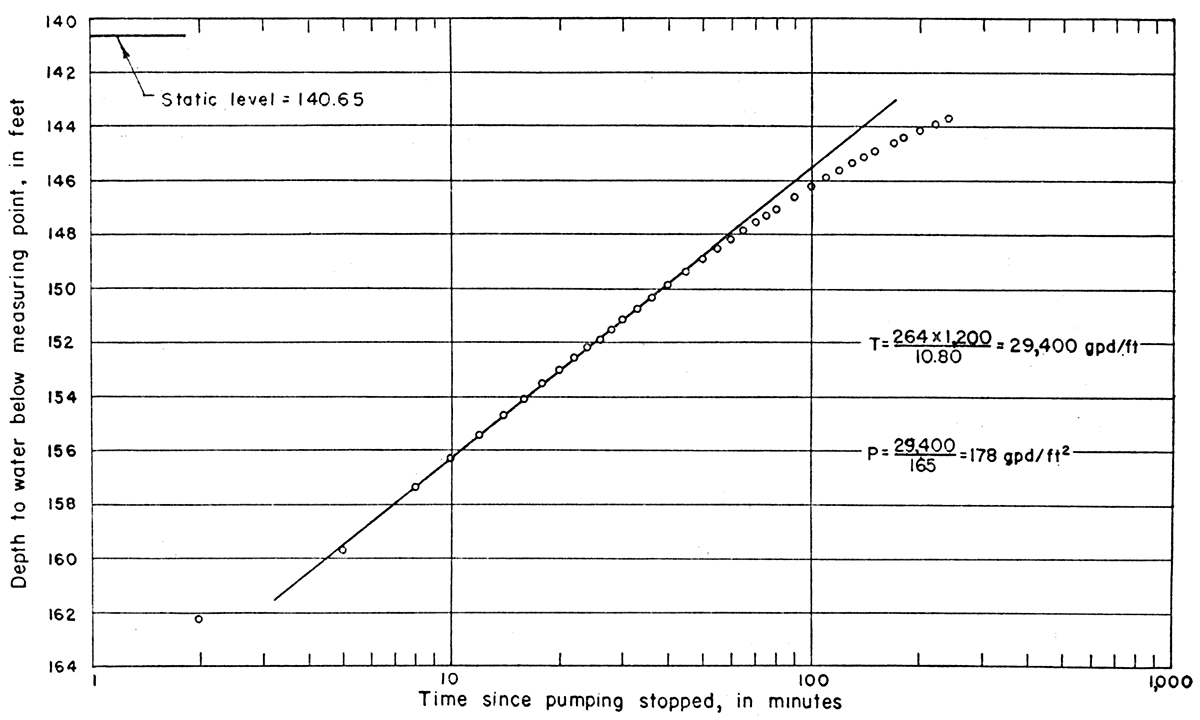
The water-level measurements made during the recovery period are listed in Table 7 and are plotted against time in Figure 25. The recovery data during the latter stage of the recovery period plotted as a curve. The earlier data plotted as a straight line and were used to compute the coefficiencts of transmissibility and permeability. By the Jacob modified non equilibrium method of computation, the coefficient of transmissibility was 29,400 gpd/ft, and the coefficient of permeability was 178 gpd/ft².

Table 7—Depth to water measured in pumped well during Clark aquifer test March 5, 1956.

Time since pumping started, in minutes	Depth to water below measuring point, in feet
8:05 a.m.	140.65 (Static)
8:30	Pump started
11:55	202.02
12:00	Pump stopped
Time since pumping stopped, in minutes	Depth to water below measuring point, in feet
2	162.20
5	159.63
8	157.32
10	156.25
12	155.38
14	154.65
16	154.05
18	153.47
20	152.98
22	152.53
24	152.16
26	151.82
28	151.45
30	151.13
33	150.71
36	150.30
40	149.84
45	149.34
50	148.88
55	148.49
60	148.13
65	147.80
70	147.51
75	147.24
80	147.01
90	146.56
100	146.19
110	145.85
120	145.58
130	145.32
140	145.08
150	144.88
170	144.52
180	144.36
200	144.10
220	143.86
240	143.64

Theoretically, the recovery data should plot as a straight line. They depart from a straight line possibly because of the lenticular structure of the water-bearing deposits in the Ogallala formation. The lower water-bearing zones have higher heads than the upper zones. Thus, during the recovery period of a well, the water comes first from all water-bearing zones. When the water level has recovered to that of the head in the zone of lowest head, the water begins to move laterally to zones of lower head and the rate of water-level recovery slows down. Consequently, the plot develops curvature as shown in Figure 25.

Figure 25—Depth to water measured in pumped well (24-30-32ca) during Clark aquifer test plotted against time since pumping stopped.

The static water level in a well penetrating and open to the full section of the Ogallala formation is not necessarily the piezometric level of any particular zone but is the resultant head of all the different zones. The differences in head indicate that the vertical permeability of the Ogallala is slight. The vertical movement of water from one permeable zone to another is retarded by less permeable zones within the Ogallala formation. In some places, these clay or silt zones may have such a low permeability that practically no water moves vertically.

C. Irsik—An aquifer test was made using an irrigation well in the NW NE sec. 14, T. 25 S., R. 29 W., on a farm owned by Clarence Irsik. The well is cased with 16-inch pipe, is 308 feet deep, and completely penetrates the Ogallala formation. It is gravel packed, and the casing is slotted throughout the saturated thickness of the formation, which is 200 feet. It was pumped April 11, 1956, at an average rate of 1,600 gpm for about 2 hours. Water-level measurements were made in the pumped well, as no observation wells were available.

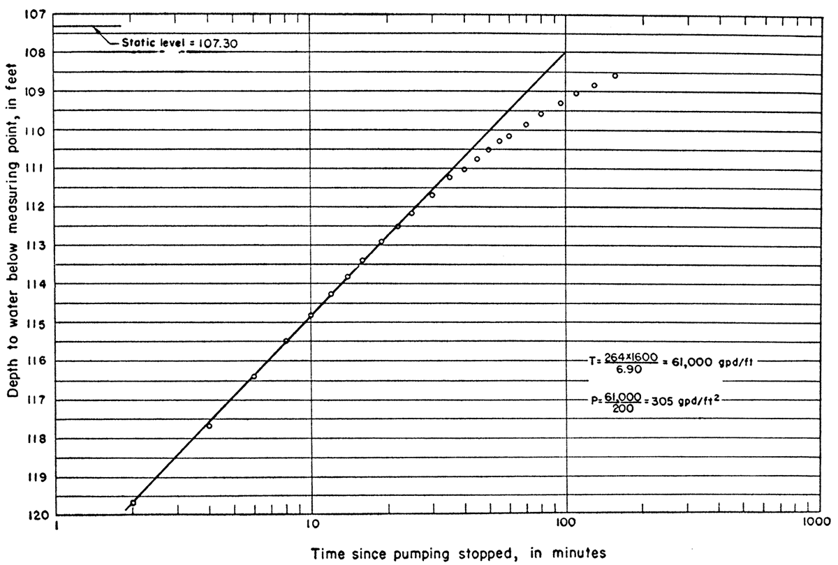
Measurements made during the recovery period are listed in Table 8 and are plotted against time in Figure 26. The recovery data departed from a straight line during the latter stage of the recovery period. The earlier data plotted as a straight line and were used to compute the coefficients of transmissibility and permeability. By the Jacob modified nonequilibrium method, the coefficient of transmissibility was 61,000 gpd/ft, and the coefficient of permeability was about 305 gpd/ft².

Table 8—Depth to water measured in pumped well during C. lrsik aquifer test April 11, 1956

Time since pumping started, in minutes	Depth to water below measuring point, in feet
8:15 a.m.	107.30 (Static)
8:50	Pump started
9:30	157.04
10:52	157.50
11:00	Pump stopped
Time since pumping stopped, in minutes	Depth to water below measuring point, in feet
2	119.66
4	117.69
6	116.39
8	115.47
10	114.79
12	114.24
14	113.80
16	113.38
19	112.90
22	112.50
25	112.16
30	111.69
35	111.21
40	111.02
45	110.73
50	110.50
55	110.28
60	110.13
70	109.82
80	109.57
95	109.28
110	109.04
155	108.57

Figure 26—Depth to water measured in pumped well (25-29-14ab) during C. Irsik aquifer test plotted against time since pumping stopped.

Summary of Aquifer Tests

The coefficients of transmissibility computed from data collected during the Ven John, Renick, and Norbert Irsik aquifer tests of the alluvium were 97,000, 181,000, and 130,000 gpd/ft, and the coefficients of permeability were 4,040, 5,040, and 5,910 gpd/ft². The lowest permeability was near the north edge of the alluvium, and the two highest were near the center of the alluvium. The average coefficient of permeability was 5,000 gpd/ft². The storage coefficients obtained from the tests of the alluvium were invalid because of slow drainage and river recharge, and a storage coefficient of 0.20 for the alluvium has been assumed.

The coefficient of transmissibility of the Ogallala formation as determined by both the McGehee and Norbert Irsik tests was about 12,000 gpd/ft, the coefficients of storage were about 2 x 10^-4 and 3 x 10^-4, respectively. These two tests showed artesian conditions in the Ogallala formation; however, near the end of the tests a recharging boundary was noted. Leakage through the confining roof or an increase in aquifer thickness, or both, may have had the effect of a recharging boundary. The evidence from well logs supports both interpretations.

The coefficients of transmissibility obtained in the Clark and C. Irsik aquifer tests were 29,000 and 61,000 gpd/ft. The reliability of the pumped-well-recovery data collected in the McGehee and Norbert Irsik Ogallala tests provides assurance that the coefficients of transmissibility obtained in the Clark and C. Irsik tests are of the right order of magnitude.

The tests show that there is better material in the Ogallala formation at the Clark and C. Irsik test sites than at the McGehee and Norbert Irsik test sites. The Clark well is on the Hank of a bedrock channel and the C. Irsik well in the middle of a bedrock channel, and in both places the lower zones contain permeable sands and gravels. Thus, the saturated thickness and transmissibility are greater than at the McGehee and Norbert Irsik sites. The McGehee well and the Norbert Irsik well are both above a bedrock high. As a result, the saturated thickness is less, and the water-bearing section does not contain the permeable sands and gravels of the lower zones.

The performances of these four wells also indicate the differences in the hydrologic properties of the Ogallala formation at the test sites. The C. Irsik well had a yield of 1,600 gpm and a drawdown of 50.2 feet after being pumped about 2 hours. The Clark well had an average yield of 1,200 gpm and a drawdown of 61.4 feet after being pumped 4 hours. The McGehee well had a yield of only 360 gpm and a drawdown of 53.5 feet after being pumped 26 hours, The Norbert Irsik well had a yield of 620 gpm and a drawdown of 68.5 feet after 24 1/2 hours.

The coefficients of transmissibility and storage obtained from data collected during the tests of the Ogallala formation indicate that pumping effects will be noted at great distances in relatively short periods of time. Wells screened in both the alluvium and the Ogallala formation should have yields of 1,000 gpm per well as long as there is a sufficient saturated thickness of the alluvium. When the alluvium becomes dewatered, the yields of wells will drop sharply.

Application of Aquifer-Test Data

Alluvium

In the Arkansas River valley, the water table slopes toward the river most of the time, and ground water consequently slowly discharges into the river. Water that is being discharged from the alluvium can be intercepted by wells before it reaches the river, and, by pumping water from storage, the gradient of the water table can be reversed so that water will move from the river toward the pumped wells. Infiltration can be induced by pumping wells near the river. The amount of water that can be obtained by induced infiltration will be determined principally by the permeability of the river bottom, by the permeability and thickness of the water-bearing materials between the river and the wells, by the quantity of flow and stage of the stream, and by the distance from the river to centers of pumping.

Water being pumped from the alluvium near Arkansas River will be replaced in part by water from the river. If pumping continues long enough, a condition of steady-state flow will result, and most or all of the water pumped will be derived from the river. Caution should be exercised in applying the coefficients of transmissibility as determined by the aquifer tests. Although recharge from the river does occur, there may be times when the stream bed is too narrow or too impermeable to allow all the available water in the river to infiltrate the aquifer even if storage space is provided below the river. As a result, some of the available stream flow may move out of the area where infiltration is needed.

The amount of infiltration that will occur in a given area will vary according to the hydraulic gradient from the river to the place of storage. After a period of no streamflow, the rate of infiltration directly below the river may be very high initially when streamflow becomes available. As a mound of water builds up beneath the river and spreads, the gradient away from the river will diminish. As a result, the rate of infiltration from the river will continue to decline as water is put back in storage, and some of the aquifer, which will be dewatered as a result of pumping during drought periods, may never be recharged with water from the river unless provision is made to divert water into those areas.

The coefficients of transmissibility and storage of the alluvium provide data for computing yield and optimum spacing of wells in the alluvium. Figure 27 shows that, after 1,000 days of pumping at a rate of 1,000 gpm, the draw down at a distance of 1,000 feet from the pumped well will be 4.7 feet, and that measurable drawdown will be noted at increasingly greater distances as pumping continues. Figure 28 shows the rate of decline caused by pumping. The drawdown in a well 1,000 feet from a well pumping 1,000 gpm for 100 days will be about 2.7 feet and for 1,000 days will be about 4.7 feet.

Figure 27—Drawdown of water level in alluvium at any distance from pumped well after pumping has begun.

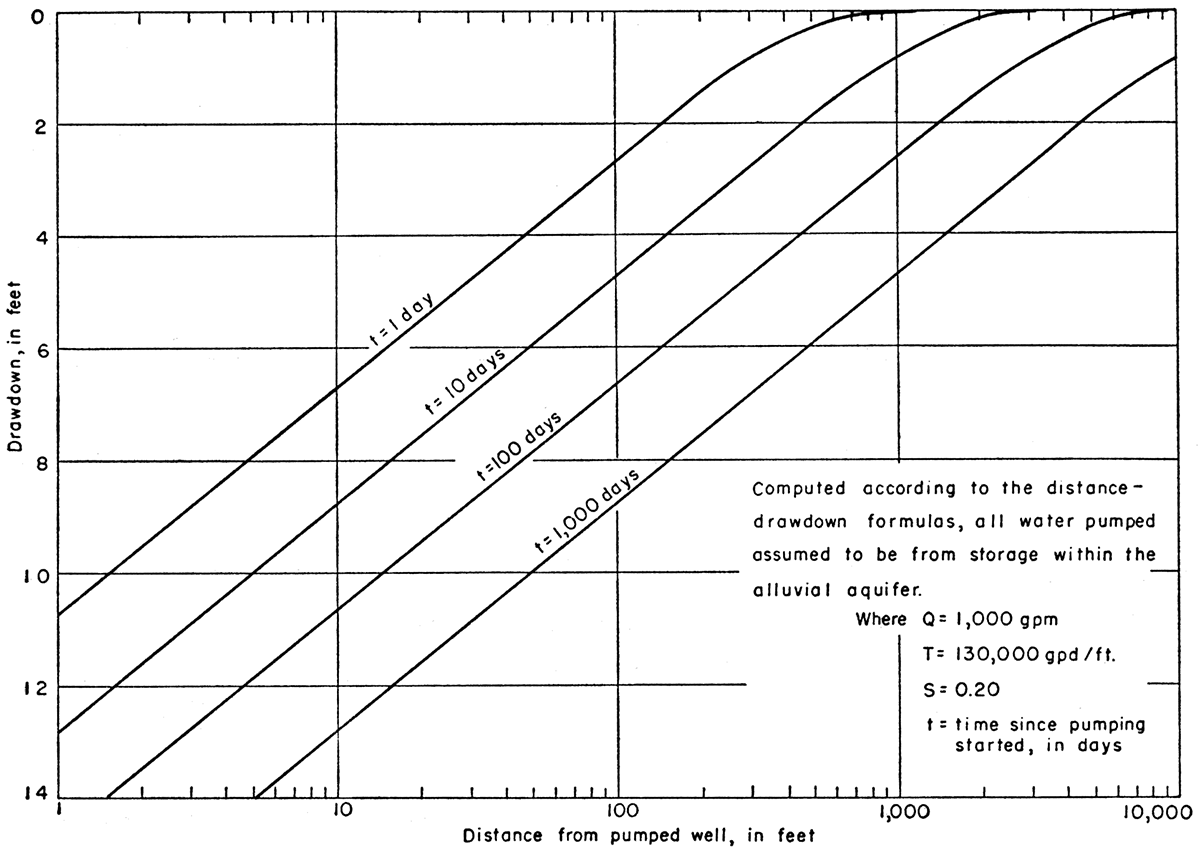
Figure 28—Drawdown of water level in alluvium at any time after pumping has begun.

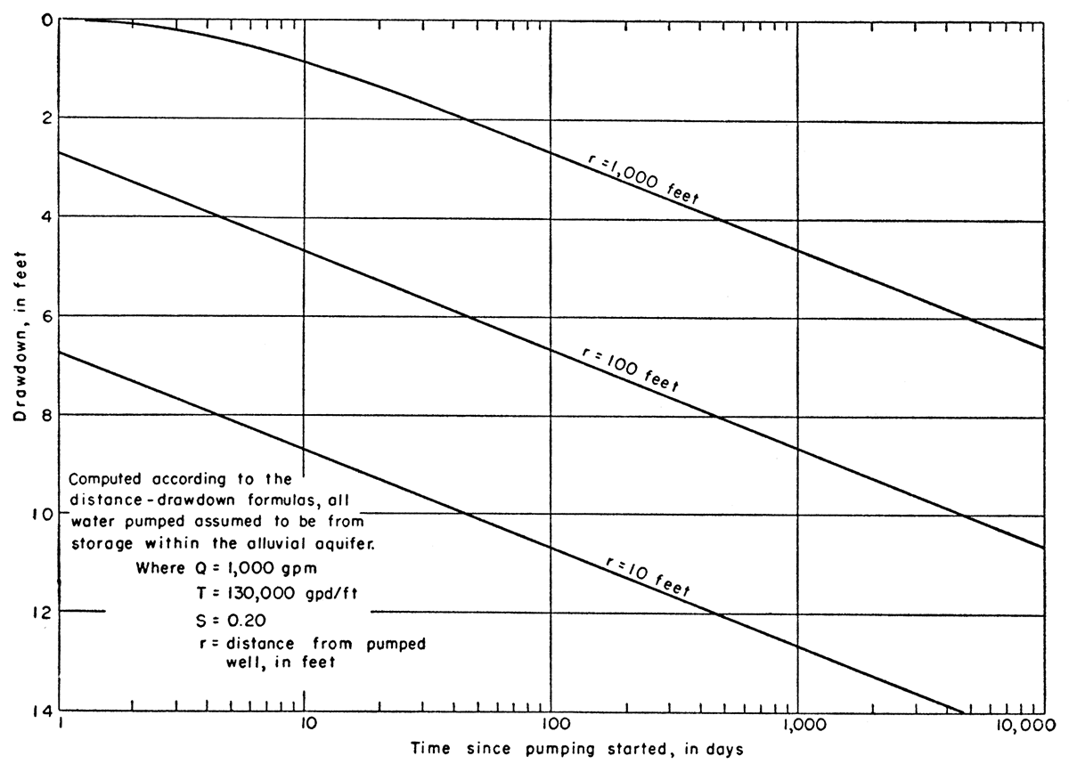
The drawdowns in Figures 27 and 28 were computed on the assumption that all water pumped came from storage in the alluvium and are given to show only the general magnitude caused by pumping. Any well placed near Arkansas River will receive recharge from it, and consequently, as long as there is water in the river, the drawdowns will be less than those shown in Figures 27 and 28. If a well is placed farther from the river and nearer the valley wall, however, the drawdowns in wells may be greater than those shown, because the alluvium pinches out. In computing declines caused by pumping from the alluvium, both the recharging effect of Arkansas River and the discharging boundary effect of the valley wall must be considered.

Ogallala Formation

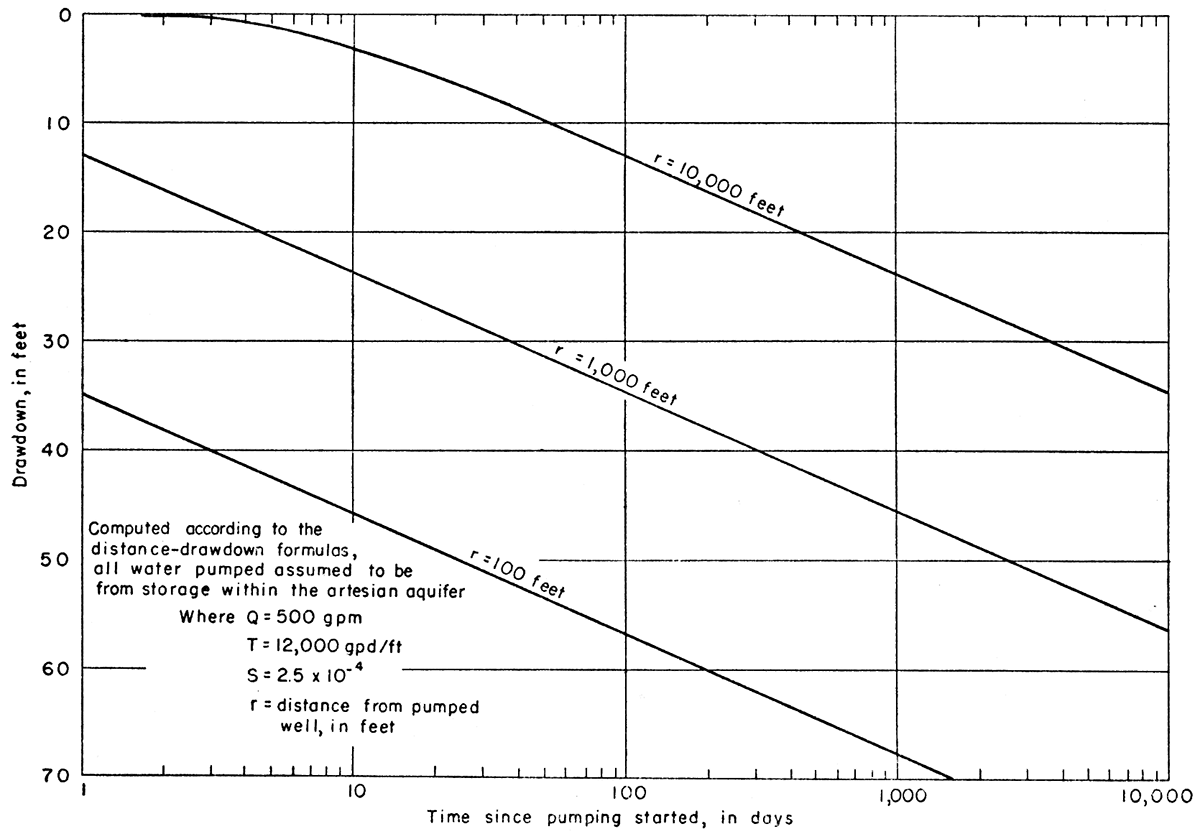
The computations for draw down in the Ogallala formation are based on the assumption that all water pumped came from storage. The drawdowns are too large because the effect of leakage and changes in lithology within the Ogallala formation have not been computed, but they show the general magnitude of decline. Figure 29 shows, under the assumed conditions specified, the drawdown of water level at any distance from a pumped well after 1, 10, 100, and 1,000 days. The data indicate that the cone of influence will spread rapidly in response to pumping in the Ogallala formation. After 100 days of pumping at a rate of 500 gpm, the drawdown at a distance of 1,000 feet will be about 35 feet. Large yields from wells cannot be maintained in the area between Pierceville and Ingalls where the permeability of the Ogallala formation is low. Also, wells pumping from the Ogallala formation in this area will seriously interfere with each other unless spaced at considerable distances. Where wells mutually interfere, the drawdown at anyone point will be the sum of the drawdowns produced by each well. Pumping lifts will increase and yields will decline. Figure 30 shows the rate of decline caused by pumping. A well pumping 500 gpm for 10 days will cause about 24 feet of decline at a distance of 1,000 feet from the pumped well, and after 1,000 days it will cause 46 feet of decline.

Figure 29—Drawdown of water level in Ogallala formation at any distance from pumped well after pumping has begun.

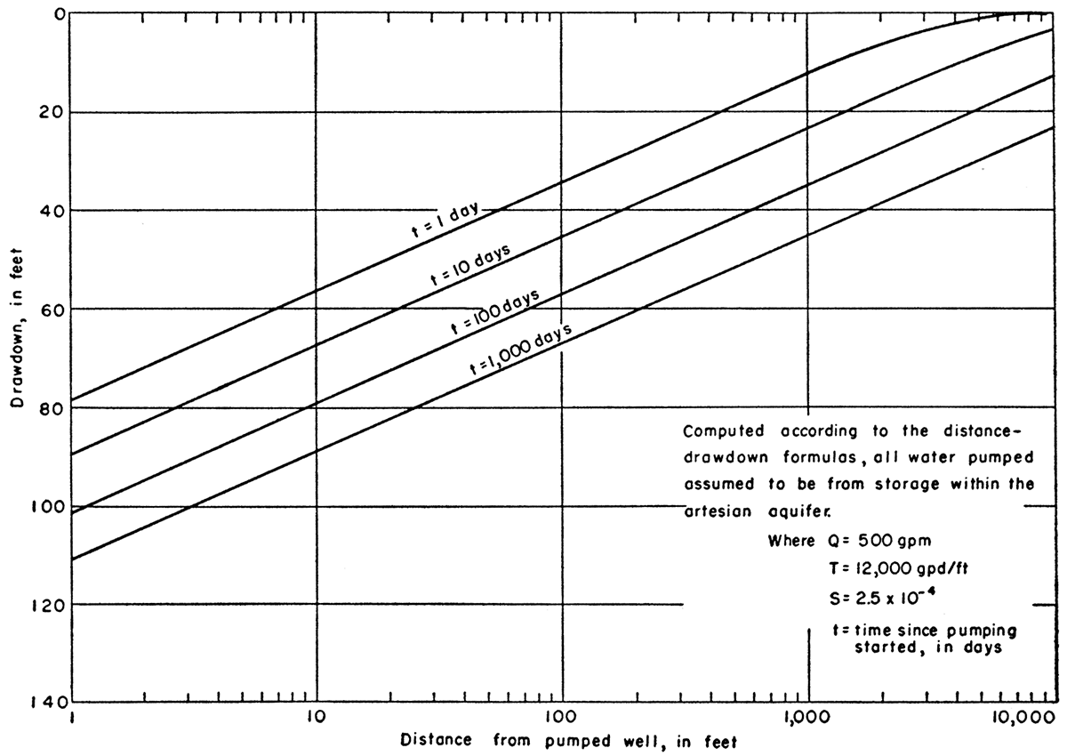
Figure 30—Drawdown of water level in Ogallala formation at any time after pumping has begun.

---

Prev Page--Ground Water Geology || Next Page--Water Table

Kansas Geological Survey, Geology
Placed on web Sept. 10, 2017; originally published July, 1958.
Comments to webadmin@kgs.ku.edu
The URL for this page is http://www.kgs.ku.edu/Publications/Bulletins/132/05_mater.html