![]()
Prev Page--Background, Construction Methods || Next Page--Discussion, Conclusions
Chapter 5--Results
Water-Level Measurements
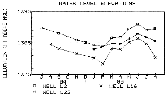
Water levels were measured in some of the wells during the study period. Some wells were measured on an almost-monthly basis while others not as regularly. In Lincolnville the average water level fluctuation was about seven feet. The lowest levels were in the winter months (usually January or February) and the highest levels were in the spring/summer months (June). The water-level hydrographs for wells L2 and L16 shown in Figure 15 represent the trends seen in other wells measured in town. Measurements for February and August 1985 in well L16 represent recovering water levels and show the drawdown effect a pumping well can have in town. The hydrograph for well L22 shows the same trend as wells L2 and L16, but only five feet of fluctuation occurred from the lowest level in January to the highest level in June (Fig. 15).
Figure 15--Water-level-elevation hydrographs for wells L2 and L16 (post-standard construction), and well L22 (pre-standard construction).
Seasonal Variations in Chemistry
Ground-water quality from wells of both pre- and post-standard construction exhibited seasonal variations during the thirteen-month study period. These variations were generally represented by decreasing and/or stabilized specific conductance and concentrations of chloride and nitrate starting in the summer and continuing through late winter. The conductance and constituent concentrations then increased through the spring and early summer, usually reaching e maximum in the May/June period coincident with increased precipitation.
The seasonal trend is exhibited by water-quality hydrographs for older (pre-1974) wells L5, L12, and L18 in Figures 16 and 17; and also by newer (post-1974) wells L2, L4, L10, and L19 in Figures 18 and 19. Newer wells L16, L20, end L21 showed only slight seasonal trends in water quality through the study period in Figure 19. Some of the small fluctuations exhibited by water quality in these latter three wells were less than the analytical error of the in-field testing equipment. Thus, the trends shown by the water-quality hydrographs for these wells may not represent true conditions.
Figure 16--Water-quality hydrographs for wells L3, L5, L12, and L26 (pre-standard construction).
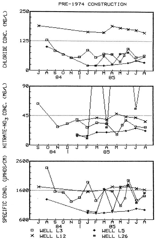
Figure 17--Water-quality hydrographs for wells L17, L18, and L22 (pre-standard construction).
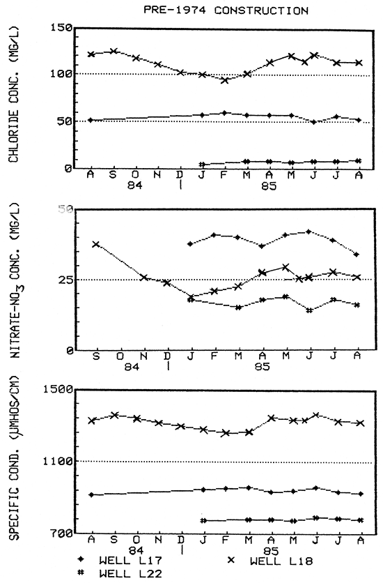
Figure 18--Water-quality hydrographs for wells L2, L4, and L10 (post-standard construction).
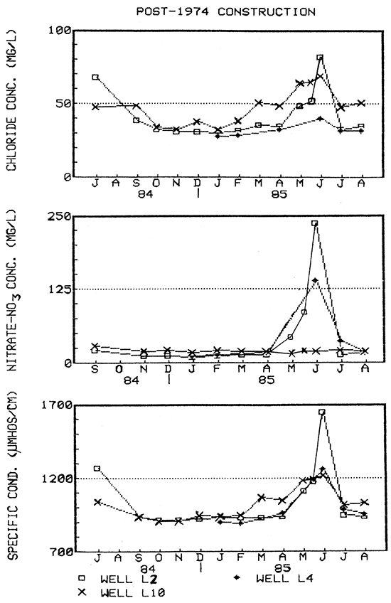
Figure 19--Water-quality hydrographs for wells L19, L20, L21, and L16 (post-standard construction).
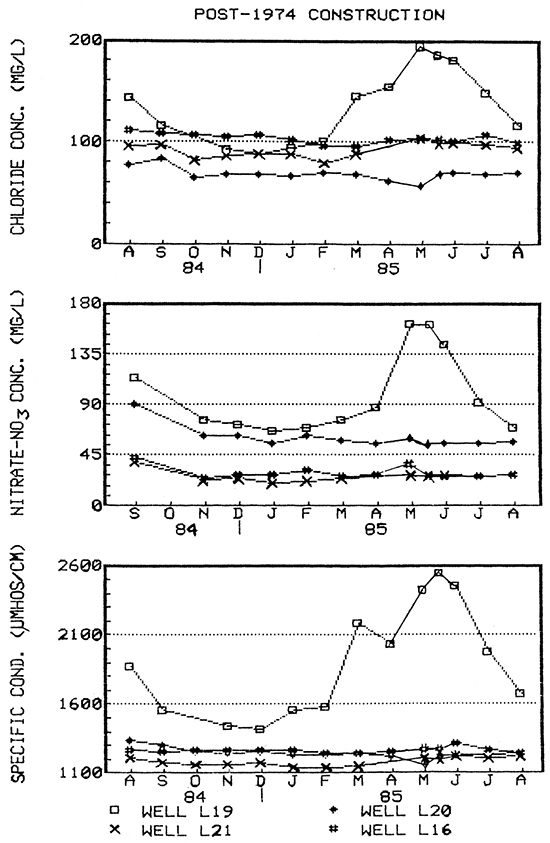
Figure 20--Water-quality hydrographs for well L15 (pre-standard construction) and Clear Creek.
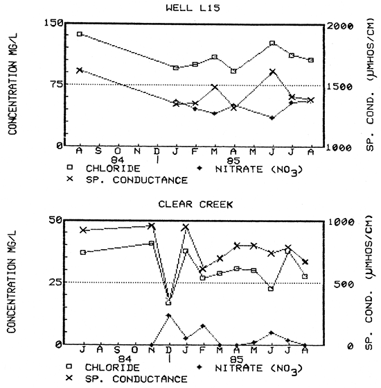
At the same time, water quality data for older wells L3, L26, and L15, showed possible seasonal trends that were partially masked by short-term fluctuations (Figs. 16 and 20). This was also the case for Clear Creek (Fig. 20), where the sporadic fluctuations were in direct response to precipitation events. However, the trend exhibited by Clear Creek of higher constituent concentrations in the winter and lower in the spring/summer months was the inverse of that exhibited by the wells. Higher discharge during the spring could have diluted higher constituent concentrations present in baseflows.
Two older wells (L17 and L22) showed little or essentially no fluctuation in ground-water quality on a seasonal basis (Fig, 17), In addition, well L22 showed only slight variation during a short-term pump test (see discussion below). No short-term water quality data was obtained for well L17.
Short-term Variations in Chemistry
Monthly Sampling
Short-term variations exhibited by some wells involved significant increases and decreases between monthly samples and usually occurred within the period May-July, Examples include: wells L2, L3, L4, L10, L19, and L26. Some of these wells also exhibited short-term fluctuations during the winter or early spring in response to precipitation as did Clear Creek.
Bi-Weekly Sampling
Because of the importance of sampling and determination of the constituents involved in the study (TOC, standard inorganic chemistry, bacteria, dissolved gases, chloride and nitrate concentrations, and specific conductance) during a spring month when precipitation was greatest, May was chosen as the month for sample collection. In order to alleviate the logistical problems associated with these sample collections, they were divided between two different sampling dates. On May 8, the eight monitoring wells were sampled for TOC (well L5 was also included) and standard inorganic chemistry analyses. On May 20, samples were collected for examination of bacteria and for determination of chloride and nitrate concentrations and specific conductance using field-testing equipment. In order to monitor ground-water quality during the month of May from other wells besides the eight monthly monitoring wells, samples were collected from five additional wells and Clear Creek on May 22 and 23, and were also analyzed for chloride and nitrate concentrations and specific conductance.
On May 6 and 7, two days before samples were collected for the TOC and inorganic chemistry analyses, a total of 3.45 inches of precipitation fell in the study area. Between the May 8 and May 20-23 sample collections, only one-half inch of precipitation fell in Lincolnville.
Table 2 shows the percent change in the constituent concentrations of ground water from the wells monitored during these two 2-week periods. Constituent concentrations in three of the six newer wells monitored (L2, L10, and L19) increased significantly within the first two-week period. One of two older wells sampled (L3) showed substantial decreases because shallow soil-water, which had seeped into the pit that the well was completed in. was overtopping the casing and flowing into the well on the day the sample was collected.
Table 2--Percent change in constituent concentration during bi-weekly sampling schedule (April-May 1985).
| Well No. |
Chloride Concentration |
Nitrate-NO3 Concentration |
Specific Conductance |
|||
|---|---|---|---|---|---|---|
| % Change 4/24-5/8 |
% Change 5/8-5/20 |
% Change 4/24-5/8 |
% Change 5/8-5/20 |
% Change 4/24-5/8 |
% Change 5/8-5/20 |
|
| L2 | 26 | 11 | 68† | 45† | 16 | 5 |
| L3* | -46 | 42 | -54 | 52 | -52 | 43 |
| L10 | 22 | 2 | -19 | 23 | 11 | 1 |
| L16 | 1 | 0 | 23 | -26 | 2 | 0 |
| L18* | 7 | -8 | 7 | -17 | -1 | 0 |
| L19 | 21 | -4 | 45† | 0† | 16 | 5 |
| L20 | -3 | 12 | 8† | -10† | -5 | 7 |
| L21 | -- | -6 | -- | -4 | -- | 0 |
| (negative values indicate a decrease in concentration) * well of pre-standard construction †this percentage change caused the nitrate concentration to exceed the U.S. EPA Interim Primary Drinking Water Standard of 45 mg/L as NO3. |
||||||
These results support the hypothesis that the Nolans Limestone in Lincolnville is rapidly recharged by precipitation leaching water-soluble constituents and contaminants from the vadose zone and ground surface. Depending on the construction and completion of the local water wells and the direction of ground-water flow, the recharge water can enter the wells and/or the Winfield aquifer and rapidly and appreciably change the water quality.
This sampling schedule in May lSB5, with respect to precipitation, also showed that some wells, namely L16, L1B, and L20, are capable of very short-term water-quality fluctuations that may not have otherwise been evident on a monthly sampling schedule.
Time-series Sampling during short-term Pump-Tests
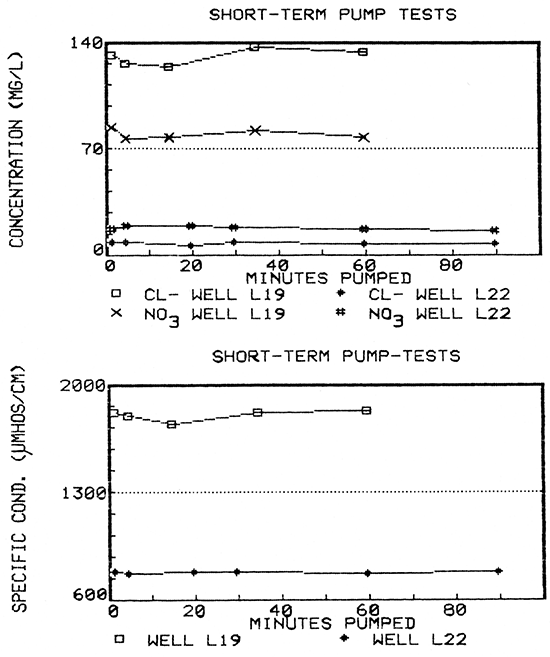
Short-term water-quality fluctuations were observed in samples collected from a newer well (L19) during a 60-minute pump-test (Fig. 21). The water quality from this well had not yet stabilized by the end of the test even though at least three well-bore volumes of water had been pumped. According to Keely (1982), the pattern exhibited by well L19, suggests not only the possibility that the well penetrated a contaminant plume and, at the same time, was experiencing a brief, localized recharge event, but also the possibility of intermittent loadings of contaminants, as might occur in karstic limestone aquifers.
Later that same day, however, when time-series sampling was conducted during a 60-minute pump-test on an older well (L22), variations in the ground-water quality remained within the analytical error (Fig. 21). In fact, the range of constituent concentrations during the pump-test (7.5-9.5 mg/L chloride; 17-20 mg/L nitrate; and 783-784 µmhos/cm specific conductance) was slightly less than the total range exhibited through the eight-month period that the well was sampled during the project (5-10 mg/L chloride; 14-19 mg/L nitrate; and 778-796 µmhos/cm specific conductance).
Figure 21--Water-quality hydrographs for wells L19 and L22 from time-series sampling during short-term pump-tests.
Total Organic Carbon
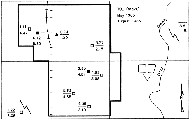
Figure 22 shows the May and August 1985 concentrations of total organic carbon (TOC) in ground water from the monitoring wells and wells LS and L22. Volatile organic carbon (VOC), and nonvolatile organic carbon (NVOC) concentrations from each well sampled are presented in Appendix VI. Because there were no detectable amounts of VOC in either sampling, the TOC concentrations shown in Figure 22 actually represent only NVOC concentrations. The fact that VOC concentrations were not detected in the May or August samplings may have been greatly affected by the sampling methods used (see Appendix V). The types of pumps used in the water wells were not conducive to sampling for volatiles and may have resulted in the loss of VOC, if present. In addition, VOC concentrations in the May samples may also have been affected by equipment malfunction in the laboratory (see Appendix VI).
Figure 22--Map of Lincolnville showing total organic carbon (TOC) in ground water from monitoring wells and wells Ls and L22 (represented by solid triangles). Samples collected May 8 and August 15, 1985. Solid symbols represent wells of pre-standard construction and open symbols represent wells of post-standard construction.
Dissolved organic carbon (DOC) is defined as the concentration of organic matter in a water sample passed through a 0.45 micrometer membrane filter. Ground water samples collected for TOC analysis in this study were not filtered prior to analysis, therefore, potentially containing both dissolved (DOC) and particulate organic carbon (POC).
The mean concentration of TOC in the May 8th sampling was 3.04 mg/L and the median concentration was 2.95 mg/L. The range of TOC concentrations in May was 0.74 to 6.12 mg/L. The mean and median TOC concentrations in the August sampling was 3.61 and 3.10 mg/L, respectively, while the range of concentrations was 1.25 to 5.80 mg/L.
With the exception of well L5, an older well, all of the wells sampled May 8th produced ground water containing TOC concentrations greater than the range found by Miller (1987) in uncontaminated ground water from consolidated aquifers in Kansas which did not exceed 1 mg/L TOC. In her study the range of TOC concentrations for all samples of uncontaminated ground water from all aquifer types in Kansas was 0.21 to 3.31 mg/L with alluvial aquifers exhibiting the highest values.
The concentrations of DOC found in uncontaminated ground water from limestone aquifers by Leenheer et al. (1974), ranged from 0.2 to 5 mg/L with a median value of 0.5 mg/L. TOC concentrations in wells L3 (pre-1974) and L19 (post-1974) exceeded 5 mg/L in the May 8th sampling, and only well L3 exceeded that level in August. The August values for wells L19 and L18 were also close to the 5 mg/L level TOC.
A wider range of DOC in ground waters (1.5-7.3 mg/L) was found in well-water supplies of five small towns in Illinois (Robinson et al., 1967).
Many of the samples exhibited an inverse relationship between TOC and NO which agreed with observations made in other studies (Miller, 1987, and Junk et al., 1980).
According to Junk et al. (1980), the absence of a significant correlation between nitrate and NVOC concentrations in the same well implies major differences in leaching and vertical transport through the unsaturated layer. The primary components of DOC are fluvic acids, which are large polymeric molecules, thus different mobilities from nitrate are to be expected.
Because of the amount of precipitation that fell in the study area prior to the May 8th sampling, discolored soil water had seeped into the well pit of well L3 and was flowing over the top of the casing directly into the well, accounting for its higher TOC concentrations. This undoubtedly would have also occurred in wells L25 and L26 or any of the other wells in the study area completed in pits. However, the concentrations of TOC in many of the other wells probably would have been higher had the samples been collected during the May 20 sampling due to potentially slower travel times for organic molecules (Junk et al., 1980).
Dissolved Gases
Concurrent with TOC analysis (as VOC and NVOC) , determinations of dissolved methane (CH4), oxygen (O2). and carbon dioxide (CO2) were made on duplicate samples collected May 8, 1985. Sampling procedures, analytical methods and results are given in Appendices V and VI. A sample collected at well L21 was accidentally broken in the laboratory and therefore no measurements of these gases are available. If VOC concentrations in any of the ground water samples had been in the detectable range (> 0.02 mg/L), it would have been necessary to determine what fraction was naturally occurring methane. The remaining fraction, therefore, would have indicated anthropogenic contamination.
Methane concentrations in the ground water samples ranged from 0.1 micrograms per liter (µg/L) in wells L5 and L18 (both older wells) to 2.7 µg/L in well L20 (a newer well), and averaged 1.1 µg/L. Figure 23 shows methane concentrations in ground water from the monitoring wells and well L5.
Figure 23--Map of Lincolnville showing concentrations of dissolved methane (CH4) in ground water from monitoring wells and well L5 (represented by the solid triangle). Solid symbols represent wells of pre-standard construction and open symbols represent wells of post-standard construction.
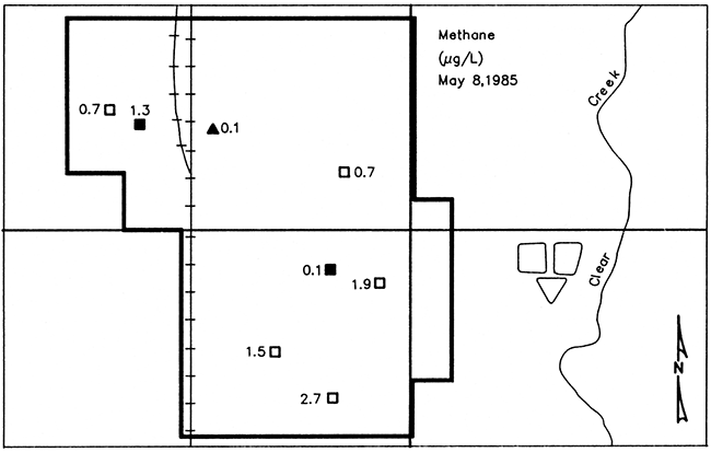
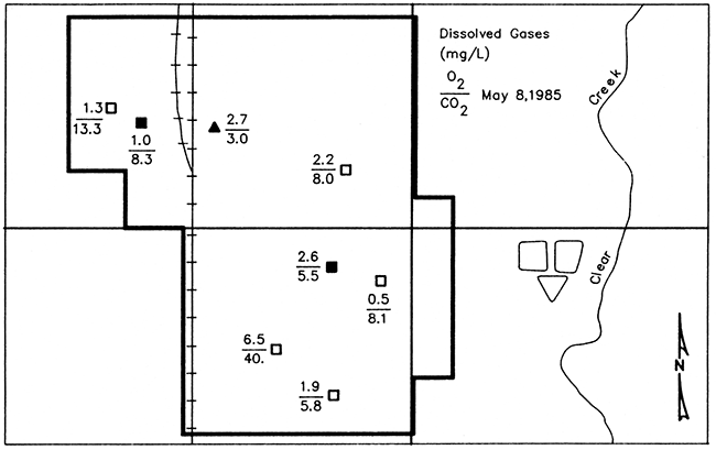
Figure 24 shows concentrations of dissolved oxygen and carbon dioxide in the ground-water samples. Dissolved oxygen concentrations ranged from 0.5 mg/L in well L16 to 6.5 mg/L in well L19, both newer wells, with a mean dissolved oxygen concentration of 2.3 mg/L. Dissolved carbon dioxide ranged from 3.0 mg/L in well Ls (pre-1974) to 40 mg/L in well L19 (post-1974), with a mean concentration of 11.5 mg/L.
Figure 24--Map of Lincolnville showing concentrations of dissolved oxygen (O2) and carbon dioxide (CO2) in ground water from monitoring wells and well L5 (represented by the solid triangle). Samples collected May 8, 1985. Solid symbols represent wells of pre-standard construction and open symbols represent wells of post-standard construction.
Standard Inorganic Chemistry
Most of the wells sampled produced CaHC03 with a few producing CaSO4 type ground waters. Results of the two standard inorganic-chemistry determinations (September 1984 and May 1985) are listed in Appendix VI. Along with the concentrations for each constituent is a calculated percentage change which, according to Summers (1972), is necessary in evaluating differences in the source of the sample when only two complete chemical analyses are available. Summers proposes that the following criteria apply in this case: If on a 1:1 comparison most concentrations have changed by at least 10 percent, significant differences have occurred in the source. If the concentration of only one constituent has changed by more than 10 percent, analysis of that constituent is suspect. If the differences are less than 10 percent, differences may exist in the source, but two analyses are not sufficient to identify them.
Wells that showed more than a 10 percent increase in most constituent concentrations from the September 1984 sampling to the May 1985 sampling were wells L2, L10, and L19 (all newer wells). Hydrographs for these wells (Figs. 18 and 19) showed the substantial increases that occur in chloride and nitrate concentrations and specific conductance during the spring. In addition, historical data from a standard inorganic analysis of a water sample collected from well L10 (June 1983), in the previous Marion County study (O'Connor et al., in preparation) is presented in Appendix VI. Figure 1 shows water quality hydrographs for well L10 during the previous county study. There was also a greater than 10 percent increase in most constituent concentrations from the September 1984 sampling to the June 1983 sampling.
Well L3 (an older well) and L20 (a newer well) showed more than a 10 percent decrease in most constituent concentrations from the September 1984 to the May 1985 standard inorganic analyses. Well L3 also showed greater than a 10 percent decrease in constituent concentrations on a short-term basis (see Figure 16 and Table 2).
Ground water from the remaining three wells (L16, L18, and L21), showed less than a 10 percent change in constituent concentrations between the September and May samplings. However, wells L16 and L18 showed a greater than 10 percent change in nitrate concentration on a short-term basis (see Figures 19 and 17, and Table 2).
Public Health Aspects
Nitrate
Nitrate values for the 13-month study period are listed in Appendix VI. Nitrate concentrations (reported as NO3) in ground-water samples from 23 of the water wells in the study area ranged from 11 to 237 mg/L. Nitrate contents of ground-water samples from the well used at the warehouse facilities, where bulk-nitrogen fertilizer and agri-chemicals were stored and handled, often exceeded 600 mg/L, with one sample (water standing in the casing) exceeding 600 mg/L. Surface water samples from Clear Creek contained from < 1 to 12 mg/L nitrate.
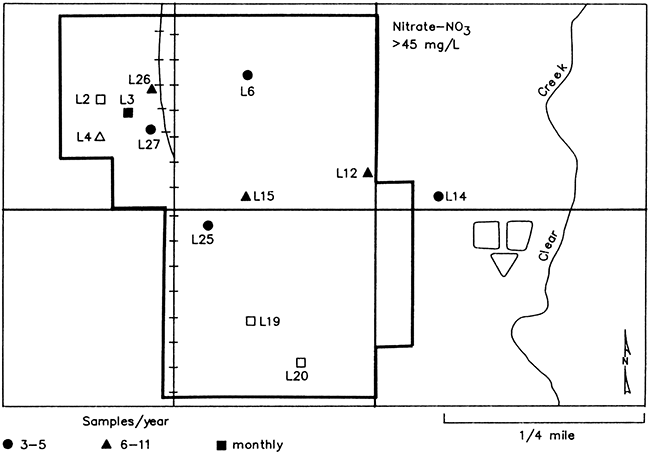
Of the 24 wells that were sampled and tested for nitrate at least once during the study period, 12 wells (50 percent) exceeded the MCL of 45 mg/L (or 10 mg/L as N), established by the U.S. EPA (Fig. 25). Four wells (16.5 percent) had been constructed since minimum well construction standards had been established in Kansas in 1974, and eight wells (33.5 percent) had been constructed or reconstructed prior to 1974.
Figure 25--Map of Lincolnville showing water wells (by well number) used in the study that exceeded 45 mg/L NO3 at least once and sampling frequency. Solid symbols represent wells of pre-standard construction and open symbols represent wells of post-standard construction.
Miller (1987) sampled 50 wells across Kansas that were either public water supply or private domestic wells for which well construction information was available. She attempted to select wells supplying uncontaminated ground water. Three of the wells (6 percent) produced ground water containing more than 45 mg/L nitrate.
In the Kansas Farmstead Well water Quality Study Heiman et al. (1987) sampled 104 farmstead wells in a random, but even distribution, across Kansas between December 1985 and February 1986. Twenty-nine percent of the wells exceeded 45 mg/L nitrate. The wells included both those constructed prior to and since the 1974 minimum well-construction standards.
Wells in this study were similar in construction to many of the farmstead wells studied by Heiman et al. (1987). Based on the seasonal and short-term variations exhibited by many of the wells in this study, it is believed that the percentage of wells in the farmstead well study producing nitrate concentrations in excess of the MCL would have been much greater if the wells had been sampled during the spring months.
Bacteria
Six of the newer wells (post-1974) and two older wells (pre-1974) were sampled in December 1984 for bacteriological examination. Fecal coliform (FC) or fecal Streptococcus (FS) bacteria were below detection limits for nearly all of the wells (Fig. 26). One exception was a sample of water siphoned back from a livestock tank into well L21 through a garden hose connected to a frost-proof hydrant lacking a back-flow preventer, thus producing a large count of fecal Streptococcus bacteria.
Figure 26--Map of Lincolnville showing fecal Streptococcus bacteria in ground water from monitoring wells sampled December 1984 and May 20, 1985. Results reported as counts per 100 mL sample. Fecal coliform bacteria were not detected. Solid symbols represent wells of pre-standard construction and open symbols represent post-standard construction.
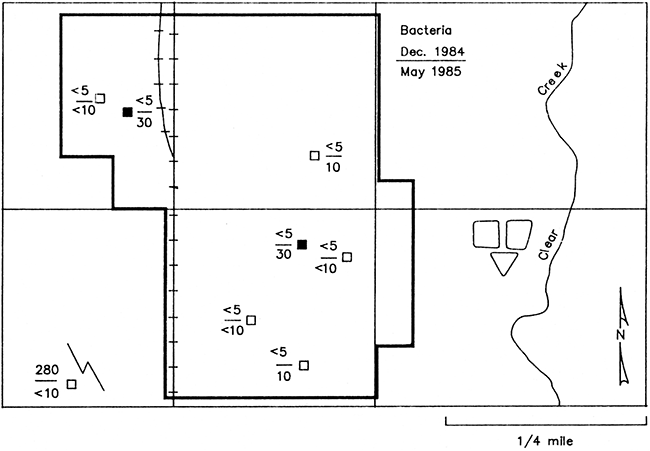
Samples collected from these wells on May 20, 1985 still showed fecal coliform bacteria below detection limits (Fig. 26). However, both of the older wells and two of the newer wells showed quantities of fecal Streptococcus greater than the one colony per 100 mL allowed by the U.S. EPA National Primary Drinking water Standards for public water supplies (U.S. EPA, 1984). The number of bacteria colonies counted might have been much higher had the samples been collected during the May 8 sampling that followed two days in which a considerable amount of precipitation fell in the study area. Research by Bitton et al. (1983) has shown that the decay rate for fecal Streptococcus bacteria is lower than for fecal or total coliform bacteria in ground water. Thus accounting for the relatively small quantities of fecal streptococcus bacteria still present in the May 20 samples.
Because the ratios of FC/FS were less than 0.7 for ground-water samples examined in this study, the source of bacterial pollution is from animal wastes (Pipes, 1982).
Prev Page--Background, Construction Methods || Next Page--Discussion, Conclusions
Kansas Geological Survey, Geohydrology
Placed on web March 16, 2016; originally published 1998.
Comments to webadmin@kgs.ku.edu
The URL for this page is http://www.kgs.ku.edu/Hydro/Publications/1988/OFR88_26/04_results.html