1. Preliminary preparations (database, budget data testing)
2. Budget variable testing and development
3. Organization and conduct of November workshop
4. Example/prototype: coral reef distribution as a test/demonstration
5. Methods development (WLV & related)
1. Cross-clustering applied to budget data
2. Measuring “success”
3. Others
6. Work and development needed before final workshop

1. Seawifs Chlorophyl-a values (C, all O cells) – cell mean and std. dev. (approx. 5’ native pixel size) for 4 years of record, all pixels, max yearly average, min yearly average. [Note:  should be treated as ocean color rather than strictly chl-a in the coastal zone; proxies for sediment, runoff, nutrients as well as primary productivity
2. Road density  (road area per land area) from Landscan data set – C and T cells.  Possible index of land use and development.
3. Temporal water flux (runoff/outflow) for the basins – max and min monthly values, intra-annual std. dev.
4. Coral Reef occurrence data (ReefBase), C and all O cells.  Number of reefs/cell, reefs yes/no (does a cell contain any reefs—binary occurrence), and a 3-value cell classification system indicating no reefs, reefs in a coastal cell with an adjacent terrestrial cell (indicator of land influence), and all other reefs (assumed ‘oceanic’ influence).
5. Single-point basin-outflow cells (coastal) for each basin – added as an option for use in budget calculations to avoid double-counting of runoff, population, etc. (NOT optimal for clustering – use original formulation).
6. Expanded selection of filters and operators for transformation and modifications to data set; data set report documenting variables used.
7. Discussion/message board on web site (single page at present; will be expanded to support multiple discussion threads with and without password control).

2.      Budget variable testing and development: 

An updated and cleaned budget variable data set was provided at the meeting [DS] and subsequently further updated [DS, SS]

New variables include system and oceanic concentrations of DIN and DIP and the value of Vx.  These are documented in the metadata file and variable list file previously sent out last week with the dataset.

Log-transformed versions of several variables were also added during the workshop, but then removed because this transformation functionality is available in the new front end.  Jeremy said that he could add these back in for the ‘canned dataset’ if this is desirable.  If there are questions about this matter, check with DS.

Budget data were loaded into the Envirodata oracle database [JB, GM] with a variable selection front that permits selection of budget variables and linking to any of the typology variables.

      This is a ‘one-to-many’ linkage, with a single set of budget variables duplicated for each of the cells that contains part of the budget site.  Considerable effort – both discussional and experimental – was expended on the problem of developing a ‘one-to-one’ linkage, in which one set of budget variables is associated with a single composite set of typology variables (e.g., averages across all of the budget cells).  This one-to-one data set might be either multi-cell (associated with all the budget-site cells) or single-cell (analogous to the basin-outflow assigned point described above).  The multi-cell approach raises the problem of assigning (e.g.) terrestrial or human dimension variable values to ocean cells that to not normally have them in the existing database and clustering approach.  The single cell approach raises similar problems if a center point us used (likely to be an O cell for the larger systems), and raises selection or representation questions if a coastal cell is used (e.g., what coastal cell should be the North Sea or Baltic representative?).  Both approaches raise concerns about compositing typology variables; simple averages may not be appropriate for many data sets or applications – for example, highly skewed data sets, variability indices (ranges or std dev), or minimum, maximum or rate/frequency data.  There is a very real possibility that averaging such numbers might lose the important signal at best (e.g., part of the system crossing a threshold value) and might be actively misleading at worst (e.g., population density on a mostly undeveloped coast with a few large cities).

      The above concerns are greatest for the larger systems, suggesting that these be avoided in the initial analysis.  Post-workshop input [SS] suggested that there are also some budget sites that are too small to be representative, and resulted in development of a list of budget sites that meet basic size and data quality criteria: this list is given in Appendix C and will be the preferred dataset for methods development and initial analysis.

      A “one-to-many” version of the data/typology spreadsheet can be created for any combination of budget and typology variables by using the new budget/typology database frontend selecting the variables as usual and then checking the ’remove nulls’ box on any budget variable before downloading the file or uploading to LOICZview.  The URL for the (presently unlinked) version of the full database front end that contains the budget variables is http://deuteron.kgs.ukans.edu/Hexacoral/envirodata/budgetdb/login_modfilt2.cfm.

      A one-to-one version of the data/typology spreadsheet can (in principle) be constructed from the one-to-many version within LOICZview (with AVERAGES of the typology variables over all typology cells corresponding to a budget site) by performing a simple supervised cluster on BUDGET ID and downloading the resulting sup file.  This sup file then contains average values of all of the variables selected.  Unfortunately, at the Swarthmore meeting, there appeared to be some kind of bug in the averaging procedure in LOICZ – this is currently being resolved.

Numerous options were discussed.  The final proposed plan is:  Three participant working groups, and three breakout ‘stations.’  Each station will have a fixed operator and facilitator, and will address a specific problem or topic area.  Stations will be networked to provide common access to interim results, resources such as Arcview files, etc., and to ensure that everyone is playing with the same deck.  To the extent possible, question formulations, draft solutions, etc., will be formulated in advance and set up to present as targets for discussion, review or modification. 

            Each working group will have a facilitator, and will rotate through all of the stations – the tentative schedule is an initial morning/noon plenary, followed by three rotational cycles of a group at a specific station for an afternoon and the following morning, followed by a lunchtime plenary for reporting and information, and a rotation.  The final afternoon will be the wrap-up plenary.

            Facilitators will be drawn from the resource people, including the regional mentors.  In addition, there will be SWAT team (Skunks With Applied Tasks) that will be called in for technical consultations and explanations within the group and that will do requested evaluation or calculational tasks needed by the groups but too time consuming to be handled by the operator. (Bruce, Dennis, maybe Jeremy, Laura, Steve?)

            Station topics should be specific, but not necessarily unique – there may be benefits in having 2 groups look at the same question from different perspectives (e.g., global and regional, tropical and temperate, etc.).  We want to be prepared to use GIS overlay  and free-standing statistical analysis in addition to LOICZVIEW – for both analysis and display/presentation.

A subset of people (CM, PS, RB) worked on developing coral reef clustering as an illustration of techniques and a test bed for method refinement.  We used the ReefBase occurrence data variables (reefcount per cell, reefs yes or no for each cell, and a classified inventory that crudely split ‘land influenced’ reefs (those in a coastal cell adjacent to a terrestrial cell) from the ‘oceanic’ (others) Results will be posted as time permits, but the major experiments and findings were:

Bruce Maxwell outlined a simple R² calculation which applies to clusters, and specifically of “dependent variables” associated with clusters (e.g. by performing a supervised cluster on the dependent variable” after having already clustered several “independent variables”).  Whether a particular variable is included in the variables cluster, or simply assigned to a cluster later by association, its mean and variance for each cluster can be calculated, the proportion of the total variance “explained” by this calculation corresponds to R².  An equivalent calculation in linear regression is often used as a measure of fit.  Dennis has written up a short summary of the calculational details and a few observations, attached as Appendix D.

An agreed goal, although not a specific immediate target, is to automate the search and refinement processes in terms of identifying “optimum” variables, weights, classes, regions, etc.

Appendix A:  Cross-clustering to relate budget and environmental variables

Note:  Cross-clustering is a semi-automated from of supervised clustering, permitting the user to generate the supervision files by clustering the “target” variables and then using those to supervise (cross-cluster) the other (typology) variables.

Procedure:

Get: Budget data set w/ typology variables (one to one), Regional/world data set w/ typology variables

Budget to World : Cluster budgets on budget variables (CLU1) Screen by latitude

                 Select actual variables to be typology variables (Important ones!!!)

                 Cross cluster Region/World using CLU1

                 Apply appropriate budget variables to each typology class and calculate
                        regional/global fluxes

World to Budget              

    Cluster world on typology (CLU2)

                 Cross-cluster budgets on CLU2

                 Overlay DDIP/DDIN/(p – r)  to see how well we did

The Experiment:

Budgets to the world

The variables: Scaled DDIN and Scaled DDIP (scaled by load)

Run MDL—   7 bumped to 10 clusters rationally there are more than 7 climate regimes

30 Runs, 50 Iterations --Select active variables to be intelligent typology variables and then cross cluster the world:

Coastal Cells, Whole world: 

Temp_CRU_Ann_avg, Precip_CRU_Total, Sub_basin_pop_density, Sub_basin_pop,SB_runoff_avgmonth, Popdensity_cellnum, Pop_tot_lsvalue, Salinity_ann_avg, Salinity_gradient, Wave_ht, Tidal_rnge, Chlora_avg_spatial, Runoff_total_ann

Cross cluster world data set based on budget clustering.  This uses as supervision points the cluster means for the typology variables that are derived from the one-to-one budget-typology data sets.  This in turn means that the input environmental variables in the first (budget) clustering are themselves means over variable numbers of typology cells associated with the various budget sites.

RESULTS: Initial trials at the workshop revealed a bug in the calculation program that rendered the results unreliable.  Corrections and further trials were conducted after the workshop.

General Discussion: How do we go from this to something useful?

We must create a subdivision of the budgets that we are happy with.

Any clustering based on the budget data is going to be noisy because of the underlying data.

This (the technique described) should be a line of questioning and exploration, but not necessarily the best way to upscale….we understand the typology variables better than the budget variables.

Driving variables of budgets

            -Budget data ret with typology variables

            -Overlay function

Improved budget clustering

            -Variable transforms

            -Data subdivision

            -“drilling in” clustering

Fluxes

            -World toBudget cross-clustering

            -Budget toWorld cross-clustering

            -Overlay of DDIN/DDIP after world budget cross-cluster

---

Appendix B

Proposed Test typology data set:  17-19 variables (ITALICIZED VARIABLES ARE NOT IN ENVIRODATA FRONT END AND MAY OR MAY NOT BE AVAILABLE); preferred testing is with transformed version (reset values and Log10), but the native values are also included.

Comment: If the mix seems to need ‘tuning’ it might be best to weight classes of variables or subsets (e.g., the water exchange parameters, the human dimension parameters) rather than working on a single variable at a time.

Issues to consider in parallel with the testing: 

---

Appendix C: Budget datasets selected for initial development and analysis (SS)

84 “Primo Budgets” for Serious Budget--Typology Intercomparison

Steve Smith (in consultation with Bob Buddemeier and Dennis Swaney)

October 17, 2001

We have agreed that some levels of limitations should be placed on the primary budget sites to use. After applying the criteria spelled out below, we presently have 84 discrete, annual budgets. A few more sites will be added, but probably not before the November workshop.

1. Sites smaller than 10 km² and larger than 20,000 km² were excluded.

a.       It is felt that, even if the budgets of the smaller systems are reliable (and many are), the meaning of the biogeochemical (nonconservative) fluxes in these small systems is likely to be very different than in larger systems. Further, at such very small spatial scales, the adjacent terrestrial influence is unlikely to be well represented by the 0.5 degree grid cells.

b.      At the other extreme, the large systems are dominated by shelf seas. These systems also seem likely to function somewhat differently than the smaller systems. Moreover, these features are likely to be linked to significantly heterogeneous terrestrial grid cells.

2. Sites deeper than 100 meters were excluded. These systems are largely functioning as small seas. Their biogeochemical cycles is likely to be dominated by surface—deep recycling, with little immediate coupling with either the land or even the deep sediments within the systems. While their budgets are often robust, both the de-coupling from land and the de-coupling from the sediments is assumed to make them very different from shallower nearshore systems.

3. Some systems also got left out because we lacked data--specifically concentration data--within the system; they were derived such that this information is difficult to pull back out (e.g., Gippsland Lakes, Australia). It may actually be possible to tease that information back out upon closer inspection.

4. Finally, the quality of budgets has been scored between 0 (bad) and 3 (very good) by SVS. It is felt that there are fatal or near-fatal flaws in those budgets scoring 0. The two most common types of flaw are clear omission of some probably important load (e.g., sewage) and such overwhelming domination by water throughput that any calculated nonconservative flux is an artifact of the calculations. While we may have a more objective criterion than the SVS scores and may want to revisit the budgets at that time, that is the only criterion we presently have in place.

These rules can be modified, and budgets will be added. But for now, the rules spell out the budgets listed.

Link to spreadsheet with budget site number, budget site name, latitude and longitude for each selected budget -- (html) (xls).

---

Notes on R² values associated with a cluster analysis

Dennis Swaney

October 15, 2001

Bruce’s approach to quantifying the proportion of the variance of any variable explained by a set of clusters should allow us to compare the clustering analysis with regressions or other analytical approaches and also to compare alternative clustering approaches. We outline the approach below.

Consider a dependent variable y, and a set of m associated independent variables, x_i, i=1,m.  If we have values of these variables for each of N cases or sample sites, we have y_j, x_ij, j=1..N.  We can perform a cluster analysis on the independent variables, creating C clusters over the N sites.  Even if we do not include the dependent variable explicitly in the cluster analysis, we still can assign the values of the y_j to each of the clusters, and calculate the mean value for each cluster , k = 1..C, and error as follows:

Mean of y in cluster k:

The “error” within cluster k is related to the variance of y within cluster k:

Overall mean and variance of y are:

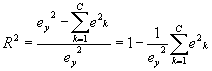
and the overall error (or sum of squared deviations) is:

A measure of the explanatory power of the clustering is given by R², equal to the total sum of squared deviations (ssd) minus the sum of square-error deviations, divided by total ssd.  Expressed in terms of the squared errors, this is:

A few observations can be made about this result, which is equivalent to the R² value used in regression, etc.