Typological Classification of

Carbonate Shelves of Caribbean

Joan Kleypas and Gerard Szejwach

see the 'readme' document for definitions and contents of folder

INTRODUCTION

The purpose of the exercise is to characterize carbonate shelves within the Caribbean region.  The initial aim was to distinguish non-carbonate from carbonate shelves, and then within the carbonate shelves, attempt to distinguish coral reef environments from non-reefal carbonate shelves (i.e., “carbonate ramps”). 

Throughout the exercise, we included both Coastal and Ocean Type I cells.  Our plan of action was to initially  explore several variables for their usefulness in distinguishing environments.  Variables were tested if they were deemed of 1) acceptable quality, 2) acceptable area coverage, and 3) either useful as a direct environmental control or as a proxy of some other environmental control.

The tested variables included:  SST (mean, min, max), Salinity (mean, min, max), Bathymetry (both ocean and land; both mean, min, max, and standard deviation), Wave Height, Tidal Range, Annual Runoff, and Annual Precipitation, Wind Speed.

Variable          Relationship to carbonate environments                  Retained?

Mean SST        possibly controls tropical carbonates                             NO

Min SST          direct control on tropical carbonates                              YES

Max SST         direct control on tropical carbonates                              NO

Mean Sal          possibly controls tropical carbonates                             NO

Min Sal            direct control on tropical carbonates                              YES

Max Sal           direct control on tropical carbonates                              NO

Mean Bathy      carbonate production limited to shallow regions NO

Min Bathy        carbonate production limited to shallow regions YES (in filtering)

Max Bathy       carbonate production higher in hydrodynamically           YES

                        exposed regions

SD Bathy         proxy for geomorphic complexity                                  NO

Wave Height    carbonate environments affected by wave energy           NO

Tidal Range      carbonate environments affected by tide energy NO

Annual runoff    proxy for water clarity, river input                                  NO

Annual Precip   proxy for water clarity                                       NO

Wind Speed     proxy for wave energy                                      NO

Initial testing and elimination of variables

We initially tested the clustering technique in the Caribbean Region (Region 10, 0-35N; 60-120W).  We quickly discovered that several variables exerted rather strong control over the clustering.  For example,  wave height had a very strong control over the clustering, mainly because all of the cells within the entire region had wave height values of 3 or 4 m.  This strongly polarized data set thus exerted undue control over the clustering.  Tidal range imposed similar weightiness in the clustering.  Both of these variables were removed from the analysis.  Annual runoff and annual precipitation were also removed from the data set.  Runoff was removed because none of the ocean cells had runoff values (logically), and annual precipitation was removed because, although precipitation within a coastal cell could serve as a proxy for water quality in that cell, precipitation over water does not impose the same influence.  Because we were interested in both coastal and oceanic I cells, we deemed these two variables as more confusing than helpful in our analysis.  Note that we recommend adding data sets that would serve as better proxies for water tranparency,such as the SeaWiFs chlorophyll or K490 data sets.

The remaining variables, SST, salinity, and bathymetry, are well-represented in the Kansas data. SST and salinity are both represented with mean, median, range, mininum, and maximum monthly values.  Bathymetry statistics include mean, minimum and maximum depths, range and also standard deviation.  We found better success at delineating carbonate shelves using SST, Salinity, and Bathymetric minima and maxima than we did using means. Because carbonate production is largely light-dependent, we used bathymetric depth as a proxy for light penetration.  Most active carbonate production does not occur in waters deeper than 30 m.  We therefore used a filter on the minimum ocean depth to limit clustering to cells where minimum depth was less than 30 m.  We also wanted to distinguish shelves which are more “exposed” to open ocean conditions from those which are more uniformly flat.  We tried two methods of identifying more “exposed” cells from the others.  One was to use standard deviation.  This highlighted cells with high bathymetric complexity. We had some success with this variable, but in the end, we found that by first filtering the depths to those less than 30 m, and then using maximum depth as a variable, we were able to distiguishing isolated and/or barrier style reefs better than with other measures of depth as a control on reef development.

RESULTS

Using this very simple list of variables (restricting data to cells with < 30m depth; and including variables maxdepth, sstmin, salmin only), we were able to distinguish carbonate shelves in the Caribbean, and within those shelves, the regions of barrier reef or most active reef growth (see summary.htm in carib_carb folder).

Carbonate shelves are indicated within most of the Caribbean, except where minimum temperatures fall below about 17degC (classes 5 – Gulf Coast, and 6 – Baja and northern). Carbonate production may also be restricted in those areas where salinity drops much below normal marine salinity of 35 PSU.  Class 2, for example, experiences an average minimum salinity of < 30 PSU.  This indicates significant  freshwater influx at least seasonally (note this corresponds to Orinoco River inputs in NE Venezuela, and high rainfall in Colombia and southern Panama).  Classes 0, 2, 7 and 6 are thus collectively called ‘non-carbonate’ shelves and comprise a total of 43% of cells.

The classes which best represent carbonate shelves in the Caribbean are: 1 (9% of cells), 3 (19%), and 4 (29%).  Of these class 1 best represents well-developed reefs, class 3 represents areas of active carbonate production, while 4 indicates the shallow flat shelves where carbonate production has a more “lagoonal” aspect (due to lower exposure to hydrodynamic conditions).  Logically, class 1 (9%) is best represented in the eastern Caribbean, and is also represented as a few “hits” in Bermuda, and the Belize Barrier Reef region.  Reef-style carbonate shelf is also sparsely represented on the Pacific coast, from Baja through Nicaragua, and in several Eastern Pacific Islands, including the Galápagos.  Notably, some reefs were clearly missed in this classification, such as Alacran reef on the Yucatan Peninsula, the Florida Keys, and portions of the Antilles Arch.  Much of the carbonate shelf region was classified as ‘moderately productive’ carbonate shelves (class 3); but the majority of the carbonate shelves occur as flat shelf areas (carbonate ramps) where carbonate sediments accumulation is probably dominated by Halimeda and red algal production.  For example, the Bahama Banks, which also includes vast shallow areas of ooid-shoals, is classified in 3.

One final interesting note here is the apparent distinctiveness of the northern Gulf of Mexico.  This segment of coastline and continental shelf persistently maintained its identity despite the number and combination of variables used.

TESTING THE CLASSIFICATION IN THE AUSTRALIAN REGION

We then tested the same relationships on a similarly sized region with similar latitudinal range to the Caribbean example:  the Australian - Indonesian (5-35S, 100-160E. See summary.htm in aus_carb folder). The Caribbean and Australian regions are actually quite similar in terms of the range and standard deviation of values for each of the three variables used.  The largest difference is in minimum salinity, with the Australian region showing similar overall salinity, but nearly twice the standard deviation and a wider range of values.

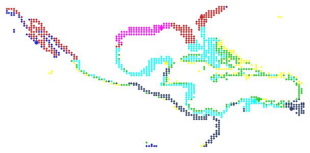
In our initial clustering of the Australian region, we failed to capture similar classifications as in the Caribbean region.  We therefore increased the number of clusters, to take into account the higher variability. This yielded better results in terms of delineating the carbonate environments.  The final ‘acceptable’ classification (at least by visual/intuitive analysis) is below:

Potential carbonate regions include classes 0, 2, 5, 6, 7, 8, 9, 10, and 11.  Most of the northwest and northeast Australian shelves classify as carbonate shelves, and the Great Barrier Reef Lagoon stands out nicely in this regard, with class 7 (dk green) delineating both the North and South sections of the GBR, and class 2 illustrating the Central GBR (set apart by a slightly lower salinity, and reflecting the probably influence of the Burdekin River).  The Barrier Reef itself is delineated by classes 0 (red) and 9 (purple).  Much of the Indonesian Archipelago and Pacific Islands were also classified as reef (0, and 9).  Coral reefs on the western coast of Australia were not distinguished in this classification.

FIRST IMPRESSIONS AND SUGGESTIONS FOR IMPROVED CLASSIFICATION

LoiczView, combined with the Hexacoral Database at the University of Kansa, provides an impressively convenient way to explore how multiple environmental parameters might control spatial distribution of environments.  We were able to quickly explore the relationship between known ecosystem types and many different environmental variables, both singly and in various combinations.  One of the best features of the system is the ‘at-your-fingertips’ availability of data sets, and the ability to automatically select variables, cell types, and regions for further analysis, or for creation of a separate multivariable data set.

The LoiczView clustering tool is an invaluable way to rapidly test whether or how environmental variables affect ecosystem.  The system operates quite robustly and provides ample information for users to examine the actual effects of the cluster analysis.  The iterative approach involved in obtaining a reasonably good fit with expected results is both a curse and a blessing.  Most in this session appeared satisfied with tuning the system slightly one way or another until a satisfactory result was used, with sometimes little thought as to why we were tuning in one direction or another (e.g., changing the number of classes, or the weighting).  This in itself was an educational experience, providing a way for testing one’s intuition, and a rather subconscious way to get a feel for both how much particular variables might be affecting environments, which variables act a reasonable proxies, etc.  This was also a quick way to test data quality.  In our case, some data sets were ignored because of insufficient coverage (runoff) or quality (wave height).  Another realization is that there are multiple “solutions” in finding the right fit of variables/weightings to a particular clustering.

Along these lines, one suggestion toward improving the system is, after selecting a suite of variables for a region, to allow one to conduct a principal component analysis on the variables.  This would provide the user with a better feel for how much influence particular variables will have  in the clustering, and would allow one to eliminate (or at least properly weight) correlated variables (e.g. temperature and surface radiation).

Keep in mind:

-         concentrating on variables that should have some reasonable affect within your region (mechanistically)

-         -data quality and coverage varies greatly between data sets; it is possible that a “proxy” data set will be better than the actual data you’re after (e.g. wind speed instead of wave height)

-         concentrate on only a few variable

-         consider eliminating or reduce weighting of covarying variables, or if you use some double measure of a variable, e.g. both min and max temperature).

JK recommends putting together a list of precautions/guidelines for users (of course I do).  All in all – this is an impressive and useful tool as long as one keeps a grasp on the logic behind the exercise.  JK also recommends the addition of some measure of light, cloudiness, and/or water transparency, as these all influence photosynthetic systems.