Coastline Complexity: A Parameter for Functional Classification of Coastal Environments
J. D. Bartley a,b,*, R. W. Buddemeier a,b, D. A. Bennett c
aKansas Geological Survey, 1930 Constant Ave., Lawrence, KS 66047, USA
bDepartment of Geography, University of Kansas, Lawrence, KS 66045, USA
cDepartment of Geography, University of Iowa, Iowa City, IA 52242, USA
Abstract
To understand the role of the world's coastal zone (CZ) in global biogeochemical fluxes (particularly those of carbon, nitrogen, phosphorus, and sediments) we must generalize from a limited number of observations associated with a few well-studied coastal systems to the global scale. Global generalization must be based on globally available data and on robust techniques for classification and upscaling. These requirements impose severe constraints on the set of variables that can be used to extract information about local CZ functions such as advective and metabolic fluxes, and differences resulting from changes in biotic communities. Coastal complexity (plan-view tortuosity of the coastline) is a potentially useful parameter, since it interacts strongly with both marine and terrestrial forcing functions to determine coastal energy regimes and water residence times, and since 'open' vs. 'sheltered' categories are important components of most coastal habitat classification schemes.
This study employs the World Vector Shoreline (WVS) dataset, originally developed at a scale of 1:250,000. Coastline complexity measures are generated using a modification of the Angle Measurement Technique (AMT), in which the basic measurement is the angle between two lines of specified length drawn from a selected point to the closest points of intersection with the coastline. Repetition of these measurements for different lengths at the same point yields a distribution of angles descriptive of the extent and scale of complexity in the vicinity of that point; repetition of the process at different points on the coast provides a basis for comparing both the extent and the characteristic scale of coastline variation along different reaches of the coast.
The coast of northwestern Mexico (Baja California and the Gulf of California) was used as a case study for initial development and testing of the method. The characteristic angle distribution plots generated by the AMT analysis were clustered using LOICZVIEW, a high dimensionality clustering routine developed for large-scale coastal classification studies. The results show distinctive differences in coastal environments that have the potential for interpretation in terms of both biotic and hydrogeochemical environments, and that can be related to the resolution limits and uncertainties of the shoreline data used. These objective, quantitative measures of coastal complexity as a function of scale can be further developed and combined with other data sets to provide a key component of functional classification of coastal environments.
Keywords: complexity; coastal morphology; habitat; classification; biogeochemical fluxes; typology
1. Introduction
The Land-Ocean Interactions in the Coastal Zone (LOICZ) project of the International Geosphere-Biosphere Programme (IGBP) has as one of its primary goals the characterization of the role of the coastal zone in global system fluxes of carbon, nitrogen and phosphorus (CNP). Since the world coastline is complex, heterogeneous, and largely unstudied, this functional globalization is being carried out by upscaling biogeochemical flux data and generalizing from well-studied areas to similar but less well-known regions (Pernetta and Milliman, 1995). This activity is being pursued with two integrated components-- the collection of validated, consistently expressed coastal biogeochemical budgets (Gordon et al., 1995; LOICZ, 2000a) and the classification of coastal systems by typology (Maxwell and Buddemeier, 2000; LOICZ 2000b).
Coastal typologies on a global scale present various challenges. First, they must depend on datasets that are truly global in coverage; second, they must adequately reflect key atmospheric, marine, and terrestrial boundary conditions and forcing functions; third, they must be able to incorporate the important effects of human populations and their environmental alterations; and finally, they must achieve some reasonable compromise between the scales and resolutions of the available datasets and the scales of the measured systems being used as type specimens.
A particular challenge in typology is acquiring and using universally available variables that reflect the nature of interactions among environmental forces, geomorphic structure, and biotic composition and function -- all of which determine flux characteristics. An initial effort within the LOICZ project collected over 30 global data sets of variables relevant to coastal studies, and organized the data into a system of coastal-zone grid cells for investigation of their utility in the coastal typology effort (http://www.nioz.nl/loicz -- link ref). As the LOICZ data collection approach evolved into a more geographically extensive system of half-degree cells and additional variables (http://www.kgs.ukans.edu/Hexacoral/Envirodata), it became apparent that specific identification and classification of the shoreline was needed. The World Vector Shoreline (Soluri and Woodson, 1990) captures the geographical form of the world's coastlines, and can be used to derive measures of coastal complexity. Coastal complexity (the degree of sinuosity or tortuosity of a coastline) is an attractive candidate for the typology project because it is widely recognized as an important modifier of both biotic community structure (e.g., Blanchard and Bourget, 1999) and water residence time. "Exposure" or "openness", a function of coastline complexity, are common criteria in habitat classification schemes.
1.3 Coastline complexity -- concepts and previous efforts
One of the first quantitative measures of coastline complexity was Mandelbrot's (1967) fractal-dimension analysis of the west coast of Britain. The fractal dimension is a measure of complexity of a statistically self-similar line -- a line that exhibits similar patterns at different scales. In most cases natural phenomena do not behave in this way. Andrle (1996) noted that the west coast of Britain has large-scale features formed by coastal submergence and tectonics (e.g., Bristol Channel and Cardigan Bay), while interspersed in these large-scale features are smaller bays, valleys, and estuaries that were formed by fluvial and glacial erosion. The application of fractals to the natural environment as a single measure of complexity is unwarranted because of their inability to differentiate between large-scale and small-scale features (Lam and Quattrochi, 1992; Goodchild, 1980; Mark and Aronson, 1984). Andrle (1994) presented a new complexity measurement routine, the angle measure technique (AMT), designed to address complexity as a function of scale. The AMT is capable of delineating changes in the complexity of geomorphic lines with scale, from which the corresponding scale of physical processes can be inferred.
One feature of the original formulation of the AMT (Andrle, 1994) is that a predetermined section of coast is used for complexity analysis. Clipping a coastline with an arbitrary grid system could lead to the breakup of key features and processes. Andrle (1996) noted that, "…complexity varies not only with scale but with position along the coastline." Attempts to clip and analyze coastlines within the LOICZ one-degree cell system revealed problems with boundary effects and artificial weighting of values due to the segmentation. This led the authors to develop and test the modified AMT described in this paper.
1.4 Objective of the study
The objective of this study was to develop, test and demonstrate a technique that would permit automated assessment of digital shorelines to determine both the extent and the scale of geometric complexity (e.g., irregularity, tortuosity, sinuosity). The output should be relevant to and usable in coastal typologies developed for the purpose of upscaling or extrapolating measured biogeochemical fluxes in specific locales to comparable environments on a global scale.
2. Methods
2.1 Case study site selection
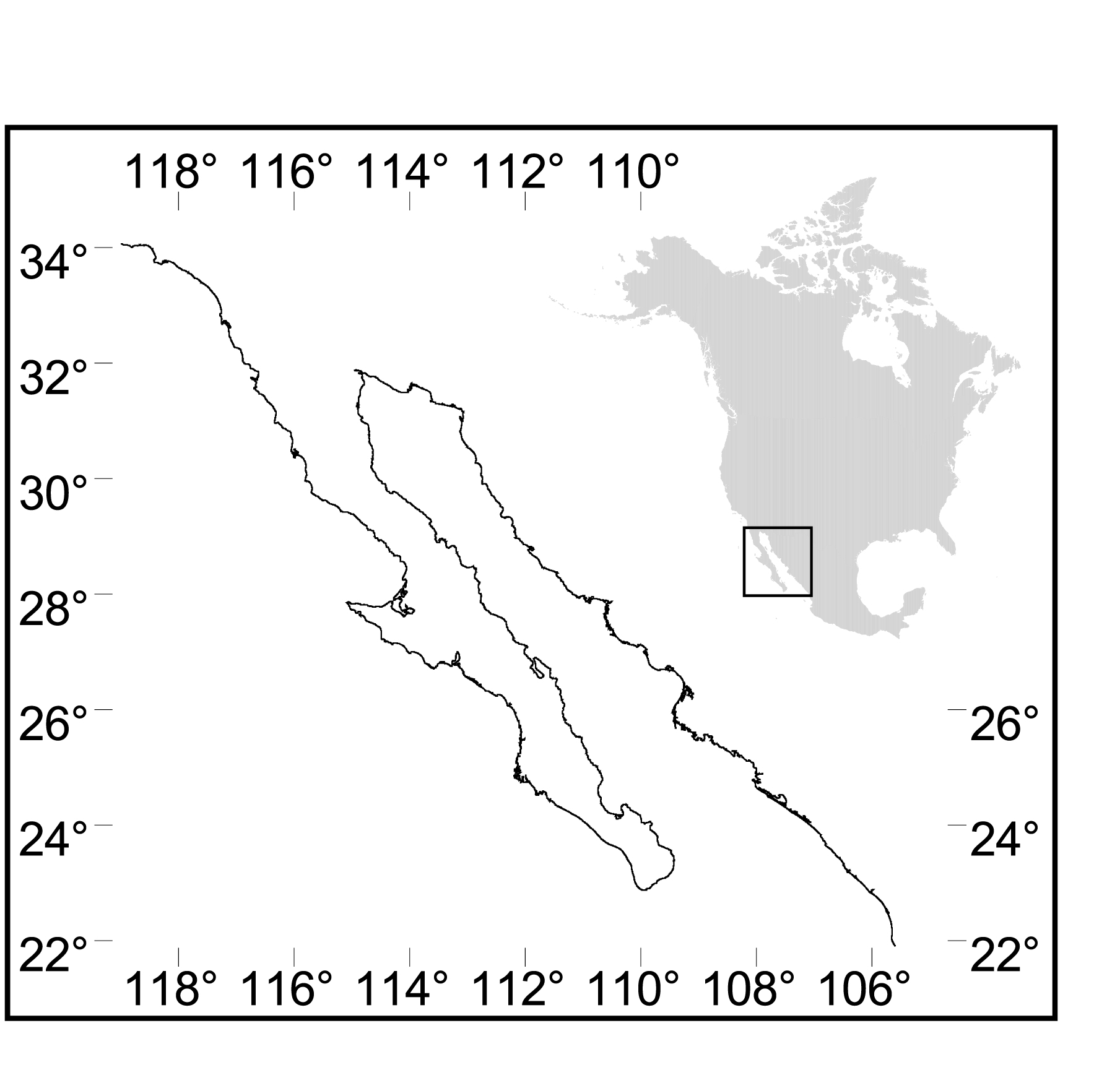
The coastline of Mexico between 34oN, 118oW and 22oN, 106oW was selected for a trial of the technique (see Fig. 1). The shoreline data set for this area (discussed below) provides a manageable number of data points and a range of point densities over a substantial length of coastline. The region has the further advantage of having a variety of marine environments, of being in a relatively data-rich area in terms of LOICZ coastal budget studies (Smith et al., 1997, 1999), and of having been part of a prior coastal classification study (Lankford, 1976).
Fig. 1. The case study area, shown with reference to its location on the North American continent.
2.2 Data used
The world vector shoreline dataset (WVS: Soluri and Woodson, 1990) was used for this study. There are higher resolution data sets available, but they are limited to well-studied regions such as Europe and the US (e.g., NOAA's Medium Resolution Digital Vector Shoreline with an average scale of 1:70,000). The WVS is the highest resolution global coastline dataset available. It has a nominal spatial resolution of about 1:250,000, but the density of points in the electronic data set varies considerably as a function of location and coastal geometry. This results in the spatial placement of points at separations ranging from 25m to 10km along the coastline, with an average separation of 1km.
2.3 The modified Angle Measurement Technique
The modification of the AMT used in this study randomly selects a specified number of points from the shoreline data set within the study area. The procedure for computing scale-dependent complexity for each of the randomly selected points is illustrated in Fig. 2. For each selected point on the coastline (A), the points of intersection between the coastline and a circle of radius S centered at A are identified. The two points of intersection separated from point A by the shortest continuous lengths of coastline are selected, and radii are drawn to them (AC and AB in Fig. 2). Angle BAD, the supplementary angle of angle BAC, is then calculated. The process is repeated for a range of values of S until a supplementary angle has been calculated for each length of interest. The supplementary angles are then plotted against the log of the length, providing a plot relating complexity (angle) on the y-axis to length (log value of S) on the x-axis. As the complexity of the coastline increases at a given scale, the angle BAD, which is the supplementary angle of angle BAC, also increases.
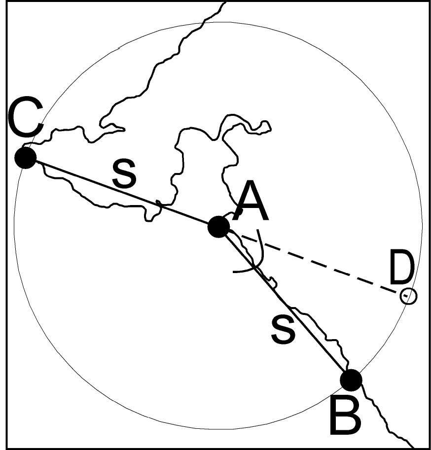
Fig. 2. Illustration of the key features in the AMT process. Angle BAD is the measure of coastal complexity at a given length scale, S. It is determined by finding the two intersections of the coastline with the radius S (points B and C) that are closest to the selected point, A, in distance along the continuous coastline. The angle of interest is the complement of the angle formed by radii AB and AC.
For the section of Mexico coastline studied, a random sample of 2.5% of the WVS shoreline points was taken (1608 out of 67089). In order to identify similar stretches of coastline, the points were clustered on the basis of similarity of the angle-log length data sets using the LOICZVIEW clustering program (Maxwell, 2000; Maxwell and Buddemeier, 2000). LOICZVIEW is a k-means clustering program specifically designed for high-dimensionality, heterogeneous data sets of the sort encountered in LOICZ typology and upscaling efforts. It produces cluster assignments, similarity indices, and identifies archetypal points that are closest to the means of each cluster. Five clusters were specified as the desired output of this particular analysis.
3. Results
3.1 Cluster archetypes and distributions
The coastal distributions of the points classified by cluster, and the archetype points for the 5 clusters selected in the LOICZVIEW analysis, are shown in Fig. 3. Also shown are expanded views of selected regions of the coast that possess high densities of points or where members of different cluster are in close proximity. One class dominates most of the coastal reaches, which is consistent both with visual inspection of the mapped shoreline and with expectations based on the relatively homogeneous geology and climate of the region. This class, represented by cluster 3, represents the straightest and ‘simplest" shoreline in the region. The other classes occur as interspersed points, reaches, or groups of heterogeneous environments.
3.2 Coastal classification
Fig. 4 shows the angle distribution plots associated with each archetype (and by extension, the distribution characteristic of the cluster). The approximate lower limit on significance (i.e., the shortest distance of S that is reliably informative) of the angle distributions, as discussed in section 4.1, is approximately one km (log S =3). Note that the archetype plots are easily distinguished in terms of both the maximum angle value(s) and the lengths at which they occur.
Fig. 3 (including the inset figures) shows the association of coastline features with the cluster members. There is generally an evident relationship between the coastline features in the vicinity of a particular point, its cluster measurement, and the angle distribution shown in Fig. 4. Also evident from the figure are gaps in the sampled coastline, the result of variations in point density in the original data set combined with the random point selection process. One of the most noteworthy issues with respect to further application is the observation that the promontories and embayments can produce the same angle distributions, but with obviously different environments (e.g., Cluster 5). This is discussed further in sections 4.2.1 and 4.3.
The most common coastal type, Cluster 3, is also the least complex, associated with relatively long, straight stretches of coastline (see archetypes and expanded views in Fig. 3). These segments tend to be the ones with the lowest point density in the data set, so the apparent simplicity at the shortest values of S may actually be in part an artifact of the data set.
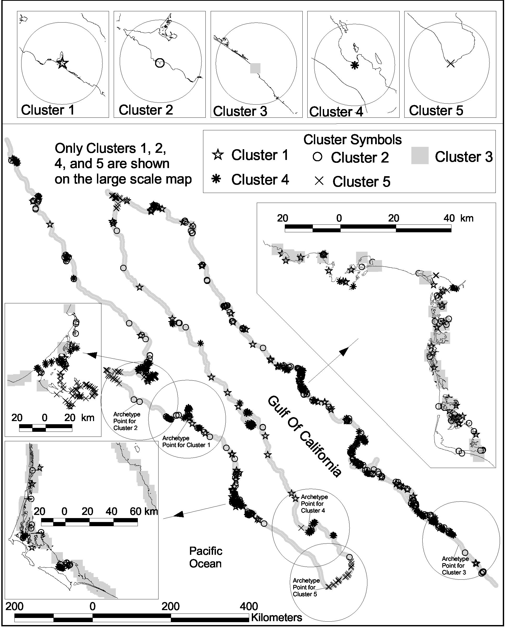
Fig. 3. Study area, with the overall distribution of cluster points and the location of the cluster archetypes shown. Upper insets show the archetype regions with other points removed for a better view of the coastline characteristics. Insets in the lower section provide expanded views of regions with high point density and/or diversity.
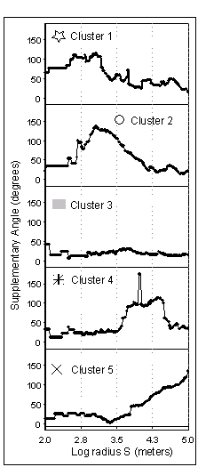
Fig. 4. Complexity plots for the five cluster archetypes shown in Fig. 3. Cluster 3 represents relatively featureless coast, while clusters 1, 2, 4, and 5 show complexity maxima at progressively greater length scales.
Clusters 1 and 2 both have complexity peaks in the one km range, but in Cluster 1 this falls off rapidly with increasing length, whereas Cluster 2 retains substantial complexity throughout the 1-10 km range. An inspection of the spatial distribution of points in these two clusters capture coastline dominated by small-scale bays and peninsulas. These two clusters seem very similar and could probably be collapsed into a single coastal class without significant loss of information. Cluster 4 has a broad complexity maximum in the 7-30 km range and represents coastal forms of moderate scale. Cluster 5 shows low complexity at short distances and steadily increasing values from 10 to 100 km -- the scale of the major landform features such as large bays and peninsulas.
4. Discussion
4.1 Limitations and generality
There is clearly no useful information in between successive shoreline points in the digital data set, and there is uncertainty about the significance of small-scale variations where points are closely spaced. This is because the transformation of field observations to maps and then to digital maps involves a succession of cartographic judgments and algorithms, both subjective and quantitative, that cannot be retrieved from the data or metadata. At resolutions comparable to the point spacing, observed patterns may say as much about the cartographer as about the coastline. There are approaches to dealing with this consideration, which should yield similar results. One is to estimate significance as a function of length based on published resolution or observed point spacings of the dataset. The other is to sample at length scales starting below the expected significance and to use the data to estimate the scale of the genuine signal.
In this situation, for example, we may hypothesize that the lower useful limit of the WVS dataset is approximately 1km, which is its mean point separation. There is, in fact, evidence in our results to support such a conclusion. All of the plots have a succession of horizontal segments at small values of S, and make a transition to smooth continuous plots in the vicinity of a one km length (3 on the log scale). Between about 2.5 and 3 on the log length scale, the flat segments have an underlying structure consistent with the patterns at slightly higher lengths. Based on these structures of the data plots (Fig. 4), it appears that the signal is relatively artifact-free above about 1.2 km in length, that there may be information in the 0.5-1.2 km range but it should be interpreted with care, and that below a few hundred meters this shoreline dataset cannot reliably provide useful results.
4.2 Relevance to other variables
Complexity by itself is a potentially informative but not conclusive variable. In order to relate it to the ecological conditions or biogeochemical function of the coast, it needs to be considered in the context of the fluxes and forcing functions that control (for example) exposure, water residence times, and material fluxes. Brandt et al. (1998) have demonstrated the importance of physical parameters in coastal classification systems. Two examples are summarized to illustrate the potential role of complexity in modulating marine and terrestrial coastal fluxes.
Fig. 5 provides examples of the relationship of complexity to the marine energy regime. At the scale of the geomorphic features, promontories and inlets of similar size will have similar angle distributions -- yet the promontory shoreline is highly exposed and the inlet shoreline, highly protected. The degree of exposure (and hence the local energy regime and water residence time) will depend on the orientation of the coastal feature with respect to prevailing winds and currents, modified by the bathymetry and presence or absence of protective barriers such as capes or islands. Bahia Sebastian Vizcaino on the west coast of Baja California is a feature that contains members of the same complexity cluster classes in obviously very different exposure settings. The map (Fig. 5) has been subjectively annotated to illustrate the probable range of exposure types. This classification process could be automated, at least for reasonably large length scales, by transforming the wind and current vector data into an onshore-alongshore coordinate system that could be combined with complexity values (at the appropriate scale) to develop an exposure index. Alternatively, subjective expert classification may be just as useful, given the levels of temporal and spatial averaging inherent in the rather coarse grid cells used for global studies.
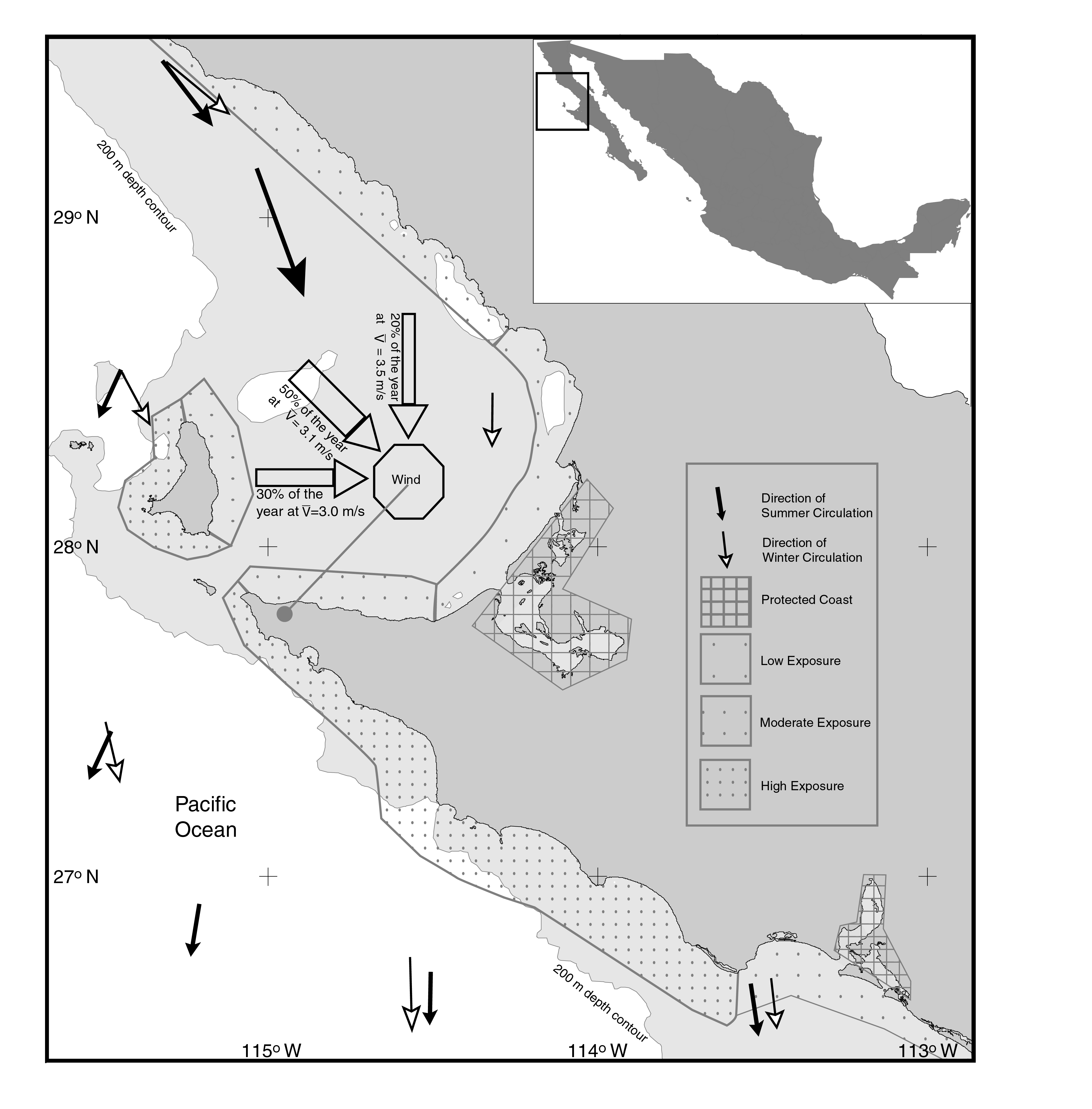
Fig. 5. Map of Bahia Sebastian Vizcaino, shown with location within the case-study area. Wind (UNAM, 1990a) and current (UNAM, 1990bc) vectors were used to develop a simple 'exposure-protection' classification that could assist in the functional interpretation of the complexity values. See Fig. 3 for the distribution of complexity cluster members within this subsystem.
Freshwater, nutrients, and sediment enter the coastal water mass from stream flow, local runoff and groundwater discharge. The association of surface water flow with the geomorphology (and consequent complexity) of estuaries and deltas is obvious (Perillo, 1995). Also potentially important in some areas is the effect of coastal configuration on groundwater discharge (Buddemeier, 1996). As illustrated in Fig. 6, groundwater flow is normal to the lines of equal potential (head), which reflect to a significant degree the land topography. This means that if inland groundwater flux is normal to the average trend of the coastline, an inlet will intercept significantly more (and a promontory, significantly less) than the fraction of groundwater discharge that would be estimated based on its mapped alongshore length. Estuaries and embayments may thus have both long residence times because of limited oceanic exchange, and enhanced input of nutrients and other materials relative to the open coast. Both factors are significant in determining ecosystem type, biological productivity, and the rate and extent of non-conservative biogeochemical processes.
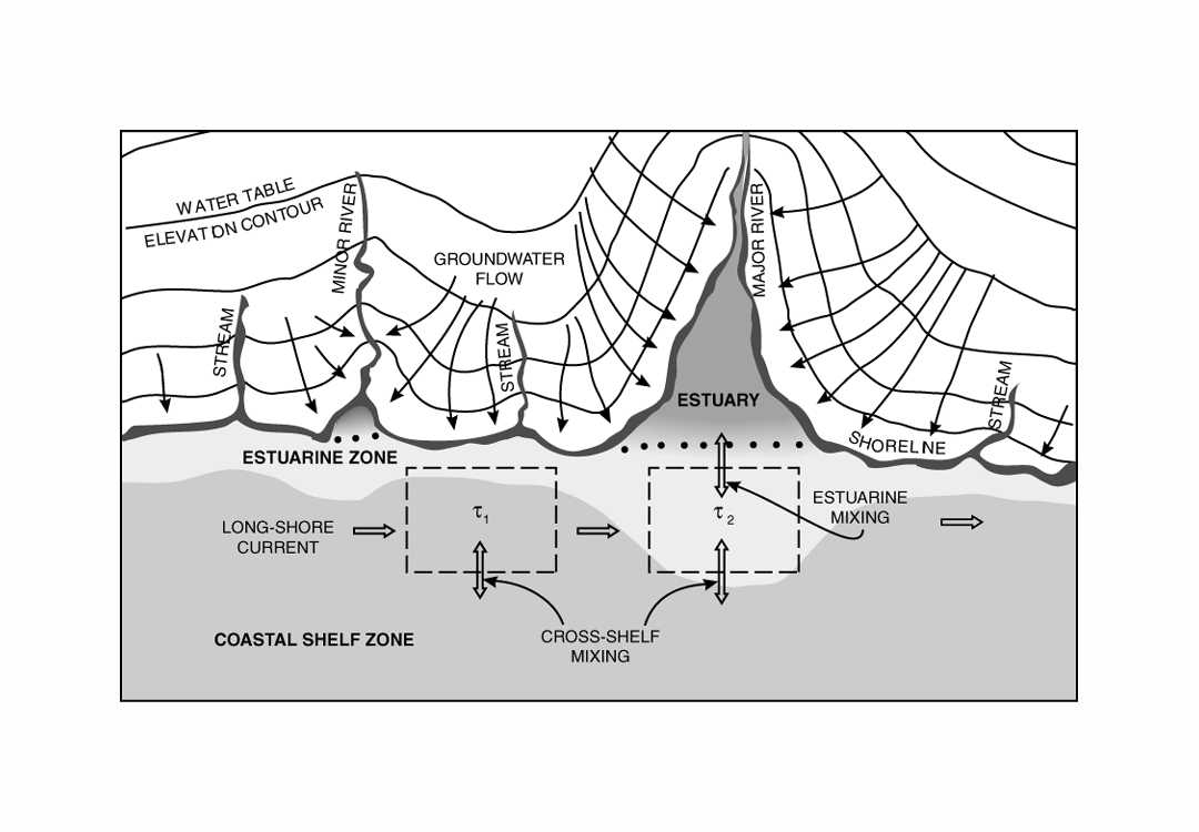
Fig. 6. Cartoon map showing groundwater discharge pathways on an irregular coastline. The 'boxes' in the estuarine zone may have similar water residence times (t ), but the chemical and biological properties of the water within them may be vastly different because of the differences in the fluxes from landward.
4.3 Further development
In addition to refinement of the computer code for ease of application and convenience of input/output, the following steps will effectively complete development of the angle-based complexity measure for application to coastal classification within the context of LOICZ objectives.
The work presented here represents a first step in the automated classification of coastal morphology through the analysis of readily available geographically referenced digital data. While this approach holds considerable promise, further refinement is required. The modified AMT procedure produces a set of relatively simple geometric indices. The interpretation of these indices in a geographical and oceanographic context is left completely to the analyst. To fully support the LOICZ global typology project we must apply the modified AMT procedure within a system that: 1) identifies geographical features (e.g., whether a point represents part of peninsulas, bay, or relatively flat coast); 2) places these features into their physical context; and 3) generalizes these data to 0.5 degree grid cells. Classifying points as peninsulas, bay, and flat coast is a relatively simple process and can be accomplished using manual or automated techniques. The modified AMT process identifies protrusions into or out from a flat coast at various scales with some success, but cannot further resolve these features into peninsulas and bays. This limitation can be easily overcome by adding simple topological relationships to the data (Peucker and Chrisman, 1975). If for example, we know that the ocean is always on the topological right of a line representing the coast, then straightforward geometrical operations can be used to distinguish a peninsula from a bay.
Understanding a location's contextual position relative to the various forcing functions that impact physical and biological processes is more problematic. The number of offshore islands within a user-specified distance can provide an initial approximation of a point's exposure to prevailing winds and currents. If such an analysis proves useful in the context of the LOICZ typology project, then more sophisticated but computationally intensive techniques may be explored. For example, through the use of topographic and bathymetric databases, each point in the coastal database can be placed within a three dimensional space. When properly oriented to applicable driving forces (e.g., climate and ocean currents) that operate over large geographical regions, it would be possible to ascertain the degree to which each point is protected by, for example, a barrier island or broad coastal flat. Such an analysis would require the development of new spatial search algorithms that would then be incorporated into the classification software. Furthermore, with the incorporation of topographic data into the analysis, the modified AMT process would be performed in both the horizontal and vertical dimension. Using these data a classification scheme could be developed that integrates morphology and geographical setting (e.g., large scale, exposed bay) and more fully represents the character of the coastline.
The generalization of spatial data is always a challenging task that requires judgment and care. Upscaling these data to the 0.5 degree grid cell level will likely present the greatest challenge of this research. To support this generalization process we will first develop a conceptual model of the critical interactions among complexity and the other variables available for use in global coastal typologies. This conceptual model will then be used to help derive statistical and knowledge-based approaches to the generalization process. To better understand the utility of this approach, empirical calibration of the complexity index by statistical experiments in geographic regions with well characterized biogeochemical budgets and a variety of coastal types will be performed. These analyses will be performed at various spatial scales and use data from various sources to assess key issues of such as portability and response to scale.
5. Summary and conclusions
Acknowledgments
We thank R. Andrle for information and advice regarding the AMT, B. A. Maxwell for his advice and assistance in the applications of LOICZVIEW, and S. V. Smith for helpful advice and discussion of the objectives and results. The support of the LOICZ IPO is gratefully acknowledged.
References
Andrle, R., 1994. The angle measure technique: A new method for characterizing the complexity of geomorphic lines. Mathematical Geology, 26(1): 83-97.
Andrle, R., 1996. The west coast of Britain: statistical self-similarity vs. characteristic scales in the landscape. Earth Surface Processes and Landforms, 21: 955-962.
Blanchard, D. and Bourget, E., 1999. Scales of coastal heterogeneity: influence on intertidal community structure. Marine Ecology Progress Series, 179: 163-173.
Brandt, A., Calman, J., and Rottier, J. R. 1998, A quantitative littoral classification system. Oceanography, 11(1): 51-57.
Buddemeier, R. W. 1996. Groundwater flux to the Ocean: Definitions, data, applications, uncertainties. in: Buddemeier, R. W. (ed.), Groundwater Discharge in Coastal Zone: Proceedings of an International Symposium. LOICZ Reports and Studies No. 8, LOICZ, Texel, The Netherlands, pp. 16-21.
Goodchild, M.F., 1980. Fractals and the accuracy of geographic measures. Mathematical Geology, 12: 85-98.
Gordon, J.D.C. et al., 1995. LOICZ Biogeochemical Modelling Guidelines. LOICZ Reports & Studies No. 5. LOICZ, Texel, The Netherlands, vi + 96 pp.
Lam, N.S. and Quattrochi, D.A., 1992. On the issues of scale, resolutions and fractal analysis in the mapping sciences. Professional Geographer, 41(1): 88-98.
Lankford, R.R., 1976. Coastal lagoons of Mexico -- Their origin and classification. in: M. Wiley (Editor), Estuarine Processes: Circulation, Sediments, and Transfer of Material in the Estuary. Academic Press, New York and others, pp. 182-215.
LOICZ, 1996. Report of the LOICZ Workshop on Statistical Analysis of the Coastal Lowlands Data Base (Typology), LOICZ Meeting Report No. 18. LOICZ, Texel, The Netherlands, pp. ii + 34.
LOICZ, 2000a. Biogeochemical Budgets Pages, Land-Ocean Interactions in the Coastal Zone. WWW Page, http://www.nioz.nl/loicz.
LOICZ, 2000b. Typology Pages, Land-Ocean Interactions in the Coastal Zone. WWW Page, http://www.nioz.nl/loicz.
Mandelbrot, B., 1967. How long is the coast of Britain? Statistical self-similarity and fractional dimension. Science, 156(5 May 1967): 636-638.
Mark, D.M. and Aronson, P.B., 1984. Scale-dependent fractal dimensions of topographic surfaces: an empirical investigation, with applications in geomorphology and computer mapping. Mathematical Geology, 11: 671-84.
Maxwell, B. A., 2000. Typology development and visualization tools for the LOICZ project. WWW Page, http://www.palantir.swarthmore.edu/~maxwell/loicz/.
Maxwell, B.A.. and Buddemeier, R.W., 2000. Coastal typology development with heterogeneous data sets. Regional Environmental Change, submitted.
NGDC, 1993. Global Relief Data on CD-ROM. National Geophysical Data Center, U. S. National Oceanic and Atmospheric Administration data set 93-MGG-01 http://www.ngdc.noaa.gov/mgg/fliers/93mgg01.html
Peucker, T. and Chrisman, N., 1975. Cartographic data structures. American Cartographer, 2:55-69.
Perillo, G.M.E. (Editors.), 1995. Geomorphology and Sedimentology of Estuaries. Elsevier, Amsterdam, 471 p.
Pernetta, J.C. and Milliman, J.D. (Editors), 1995. Land-Ocean Interactions in the Coastal Zone: Implementation Plan. IGBP Report No. 33. IGBP, Stockholm, 215 pp.
Smith, S.V., Ibarra-Obando, S., Boudreau, P.R. and Camacho-Ibar, V.F., 1997. Comparison of Carbon, Nitrogen and Phosphorus Fluxes in Mexican Coastal Lagoons, LOICZ Reports & Studies No. 10. LOICZ, Texel, The Netherlands., pp. ii + 84.
Smith, S.V., Dupra, V., Marshall Crossland, J.I. and Crossland, C.J., 1999. Mexican and Central American Coastal Lagoon Systems: Carbon, Nitrogen and Phosphorus Fluxes (Regional workshop II), LOICZ Reports & Studies No. 13. LOICZ, Texel, the Netherlands, pp. ii + 115 pp.
Soluri, E.A. and Woodson, V.A., 1990. World vector shoreline. International Hydrographic Review, LXVII(1): data available in Global Relief Data on CD-ROM (1993), National Geophysical Data Center, U. S. National Oceanic and Atmospheric Administration data set 93-MGG-01. (http://www.ngdc.noaa.gov/mgg/fliers/93mgg01.html)
UNAM (Universitad Nacional Autónoma de México), 1990a. Viento Dominante Durante el Año. In: Atlas Nacional de México, Instituto de Geografía, UNAM, Mexico City, map IV.4.2.
UNAM (Universitad Nacional Autónoma de México), 1990b. Oceanografía Física 1. In: Atlas Nacional de México, Instituto de Geografía, UNAM, Mexico City, map IV.9.1.
UNAM (Universitad Nacional Autónoma de México), 1990c. Oceanografía Física 2. In: Atlas Nacional de México, Instituto de Geografía, UNAM, Mexico City, map IV.9.2.